Introduction to Machine Learning

CMSC 173 - Module 00

Noel Jeffrey Pinton
Department of Computer Science
University of the Philippines Cebu

Course Overview

Topics Covered
What is Machine Learning?
Types of Learning: Supervised, Unsupervised, Reinforcement
The ML Pipeline
Bias-Variance Tradeoff
Best Practices & Ethics

What is Machine Learning?

Formal DefinitionMachine Learning (ML) is the science of getting computers to learn and act like humans do, and improve their learning over time in autonomous fashion, by feeding them data and information.

Key CharacteristicsLearning from data without explicit programming
Improving performance with experience
Discovering patterns in complex datasets
Making predictions or decisions

Traditional Programming vs ML

Traditional:\\ Rules + Data → Answers Machine Learning:\\ Data + Answers → Rules

Core Insight

ML finds the rules automatically from examples!

Traditional Programming vs ML

AspectTraditionalMachine Learning

InputRules + DataData + Labels
OutputAnswersRules/Model
Exampleif price > 1000: expensiveLearn threshold from examples

Aspect	Traditional	Machine Learning
Input	Rules + Data	Data + Labels
Output	Answers	Rules/Model
Example	if price > 1000: expensive	Learn threshold from examples

Historical Context

"A computer would deserve to be called intelligent if it could deceive a human into believing that it was human." --- Alan Turing

Major Milestones1950s: Alan Turing - "Can machines think?"
1957: Perceptron (Frank Rosenblatt)
1986: Backpropagation popularized
1990s: Support Vector Machines
1997: Deep Blue defeats Kasparov
2006: Deep Learning renaissance
2012: AlexNet wins ImageNet
2016: AlphaGo defeats Lee Sedol
2020s: Large Language Models

The Three AI Winters

Periods of reduced funding and interest:

1970s: Perceptron limitations
1987-1993: Expert systems fail
Post-2000: AI hype deflation

Current Era

We're in the Deep Learning Revolution:

Big data availability
GPU acceleration
Novel architectures (Transformers)
Widespread deployment

Real-World Applications

"Machine learning is the last invention that humanity will ever need to make." --- Nick Bostrom

Computer VisionMedical image diagnosis
Autonomous vehicles
Facial recognition
Object detection & tracking
Image generation (DALL-E, Midjourney)

Natural Language ProcessingMachine translation
Chatbots & virtual assistants
Sentiment analysis
Text summarization
Question answering

Other DomainsFinance: Fraud detection, trading
Healthcare: Drug discovery, medicine
E-commerce: Recommendations
Gaming: AI opponents
Manufacturing: Quality control
Agriculture: Crop monitoring

Impact

ML is transforming every industry!

Learning Objectives

By the end of this course, you will be able to:Understand the fundamental concepts and mathematical foundations of machine learning
Distinguish between different types of learning paradigms (supervised, unsupervised, etc.)
Implement core ML algorithms from scratch using Python
Apply appropriate ML techniques to real-world problems
Evaluate model performance using rigorous metrics
Analyze the theoretical properties of learning algorithms
Compare different approaches and select optimal methods
Understand state-of-the-art techniques in deep learning

Prerequisites

CMSC 170: Linear algebra, probability theory, calculus, Python programming

Machine Learning Taxonomy

See visual diagram in lecture materials

Supervised Learning

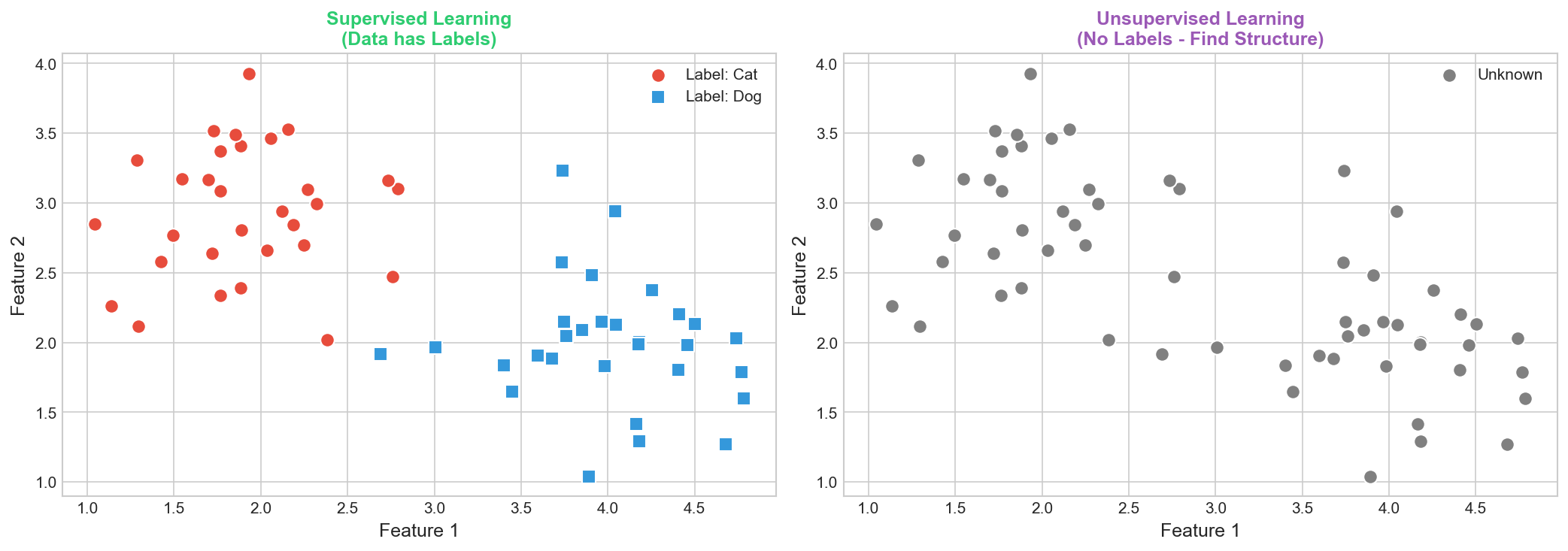
Definition: Learning from labeled data

Input: $\mathbf{x} \in \mathbb{R}^d$
Output: Label $y$
Goal: Learn $f(\mathbf{x}) \approx y$

            Two Main Tasks
            Regression: $y \in \mathbb{R}$
Classification: $y \in \{1,...,K\}$

        

Supervised Learning: Training

Training Process

Given $\mathcal{D} = \{(\mathbf{x}_i, y_i)\}_{i=1}^n$:

Choose hypothesis class $\mathcal{H}$
Define loss $\mathcal{L}(y, \hat{y})$
Minimize empirical risk:
$$\hat{f} = \arg\min_{f \in \mathcal{H}} \frac{1}{n}\sum_{i=1}^n \mathcal{L}(y_i, f(\mathbf{x}_i))$$

Key Properties

Labeled data required
Teacher signal guides learning
Generalization to new examples

Challenge

Avoid overfitting to training data!

Python Example

from sklearn.model_selection import train_test_split
from sklearn.linear_model import LogisticRegression

X_train, X_test, y_train, y_test = train_test_split(X, y, test_size=0.2)
model = LogisticRegression().fit(X_train, y_train)
print(f"Accuracy: {model.score(X_test, y_test):.2f}")

Regression: Predicting Continuous Values

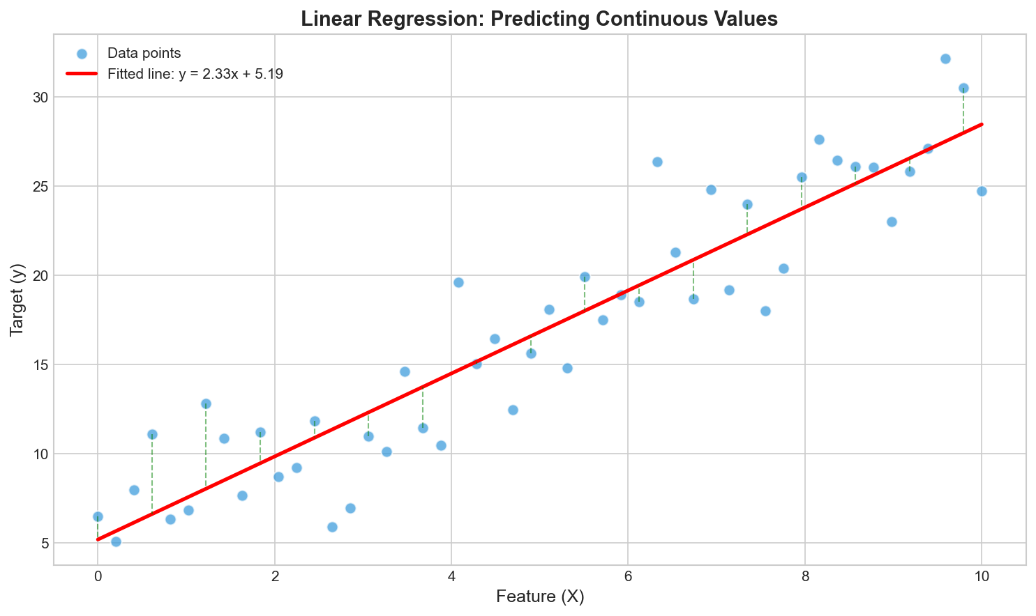
Regression Example — Linear Regression with Fitted Line

Input: $\mathbf{x} \in \mathbb{R}^d$
Output: $y \in \mathbb{R}$ (continuous)
Model: $\hat{y} = f(\mathbf{x}; \theta)$

            Loss Functions
            MSE: $\frac{1}{n}\sum (y_i - \hat{y}_i)^2$
MAE: $\frac{1}{n}\sum |y_i - \hat{y}_i|$

        

Regression: Algorithms & Examples

            Regression Algorithms
            Linear Regression
Ridge/Lasso (regularized)
Polynomial Regression
SVR, Decision Trees
Neural Networks

        

Real-World Examples

House price prediction
Stock forecasting
Temperature prediction
Sales forecasting

Python Example

from sklearn.linear_model import LinearRegression
from sklearn.metrics import mean_squared_error, r2_score

model = LinearRegression().fit(X_train, y_train)
y_pred = model.predict(X_test)
print(f"MSE: {mean_squared_error(y_test, y_pred):.4f}")

Classification: Predicting Categories

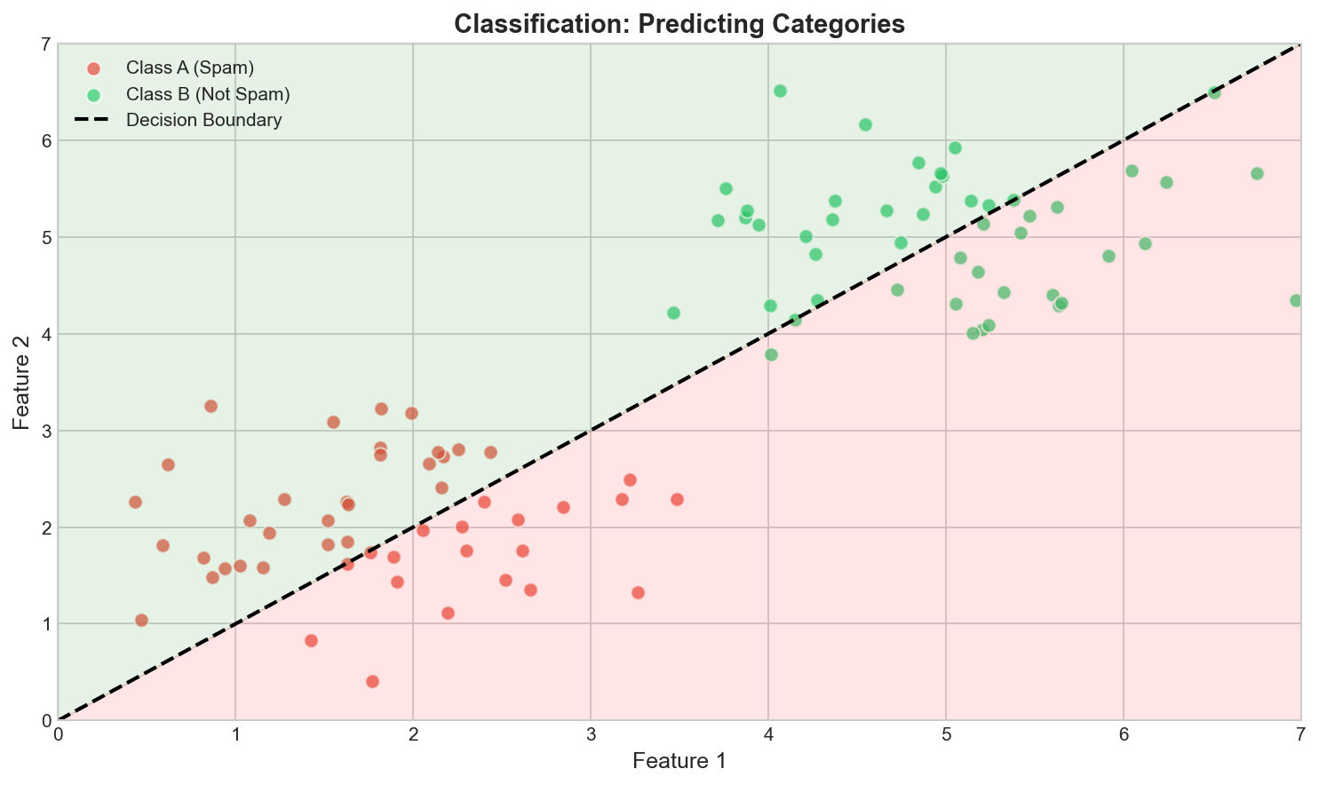
Classification Example — Decision Boundary Separating Classes

Input: $\mathbf{x} \in \mathbb{R}^d$
Output: $y \in \{1,...,K\}$ (discrete)
Model: $\hat{y} = \arg\max_k P(y=k|\mathbf{x})$

            Types
            Binary: $K=2$ (spam/not spam)
Multi-class: $K>2$ (digits 0-9)
Multi-label: Multiple tags per item

        

Classification: Algorithms & Code

            Classification Algorithms
            Logistic Regression
Naive Bayes
K-Nearest Neighbors
Decision Trees
Random Forests, SVM

        

Loss Functions

Cross-Entropy:

$$\mathcal{L} = -\frac{1}{n}\sum_{i} y_i \log \hat{y}_i$$

Hinge Loss (SVM):

$$\mathcal{L} = \max(0, 1 - y\hat{y})$$

Python Example

from sklearn.ensemble import RandomForestClassifier
from sklearn.metrics import classification_report

clf = RandomForestClassifier(n_estimators=100).fit(X_train, y_train)
print(classification_report(y_test, clf.predict(X_test)))

Unsupervised Learning

DefinitionLearning from unlabeled data without explicit target outputs:
Input: Feature vectors $\{\mathbf{x}_1, …, \mathbf{x}_n\}$
Output: None (discover structure)


Goal: Discover hidden patterns, structures, or relationships in data

Main Tasks1. Clustering
Group similar data points
Algorithms: K-Means, DBSCAN, Hierarchical


2. Dimensionality Reduction
Compress high-dimensional data
Algorithms: PCA, t-SNE, UMAP


3. Density Estimation
Model the data distribution
Algorithms: Gaussian Mixture Models

Key Characteristics

No labels required
Exploratory in nature
Structure discovery
Performance harder to measure

Applications

Customer segmentation
Anomaly detection
Data visualization
Feature extraction
Compression
Recommender systems

Challenge

How do we evaluate without labels?

Supervised vs Unsupervised Comparison

AspectSupervisedUnsupervised

DataLabeled (X, y)Unlabeled (X only)
GoalPredict y from XFind hidden patterns
EvaluationCompare to true labelsInternal metrics
ExamplesClassification, RegressionClustering, PCA

Aspect	Supervised	Unsupervised
Data	Labeled (X, y)	Unlabeled (X only)
Goal	Predict y from X	Find hidden patterns
Evaluation	Compare to true labels	Internal metrics
Examples	Classification, Regression	Clustering, PCA

Clustering: Grouping Similar Data

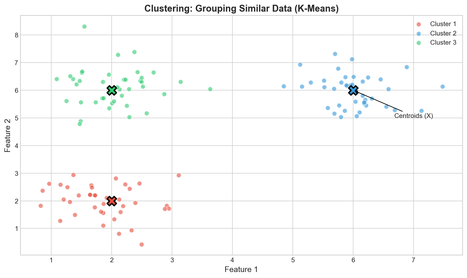
K-Means Clustering — K-Means with 3 Clusters

Goal: Group similar data points without labels

            K-Means Objective
            $$\min \sum_{i=1}^n \|\mathbf{x}_i - \mu_{c_i}\|^2$$
            Initialize K centroids
Assign points to nearest
Update centroids
Repeat until convergence

        

Clustering: Methods & Evaluation

            Other Clustering Methods
            Hierarchical: Dendrogram
DBSCAN: Density-based, finds arbitrary shapes
GMM: Probabilistic, soft assignments

        

Evaluation Metrics

Silhouette coefficient
Davies-Bouldin index
Calinski-Harabasz index

Python Example

from sklearn.cluster import KMeans
from sklearn.metrics import silhouette_score

kmeans = KMeans(n_clusters=3).fit(X)
score = silhouette_score(X, kmeans.labels_)
print(f"Silhouette: {score:.3f}")

Dimensionality Reduction

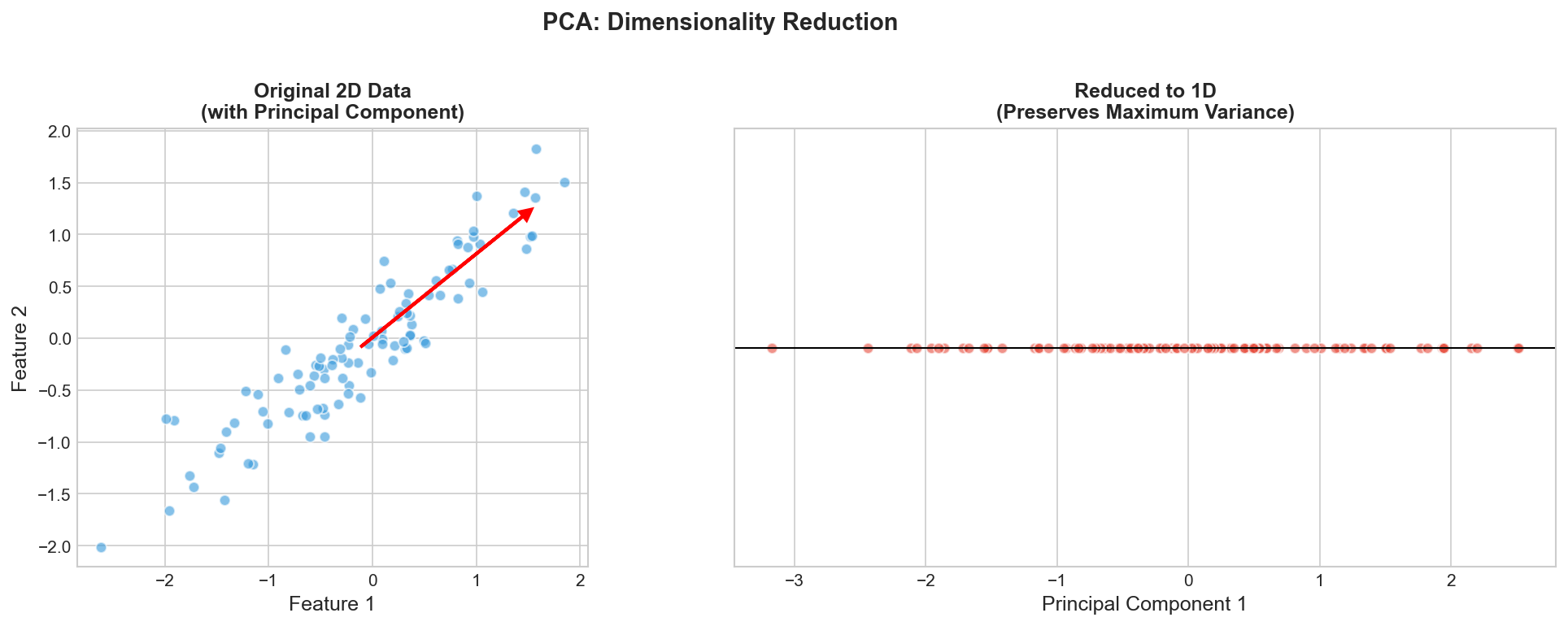
PCA Visualization — PCA: Principal Components

Goal: Compress high-dim data while preserving structure

            Curse of Dimensionality
            Volume grows exponentially
Data becomes sparse
Overfitting risk increases

        

PCA & Other Techniques

            PCA Algorithm
            Center data: $\tilde{\mathbf{x}}_i = \mathbf{x}_i - \bar{\mathbf{x}}$
Compute covariance: $\mathbf{C} = \frac{1}{n}\mathbf{X}^T\mathbf{X}$
Find eigenvectors of $\mathbf{C}$
Project onto top $k$ eigenvectors

        

Other Techniques

Linear: PCA, LDA, ICA
Non-linear: t-SNE, UMAP
Neural: Autoencoders

Python Example

from sklearn.decomposition import PCA

pca = PCA(n_components=2).fit(X)
X_reduced = pca.transform(X)
print(f"Variance explained: {pca.explained_variance_ratio_.sum():.2%}")

Semi-Supervised Learning

DefinitionLearning from both labeled and unlabeled data:
Labeled: $\mathcal{D}_L = \{(\mathbf{x}_1, y_1), …, (\mathbf{x}_l, y_l)\}$
Unlabeled: $\mathcal{D}_U = \{\mathbf{x}_{l+1}, …, \mathbf{x}_{l+u}\}$
Typically $l \ll u$ (few labels, many unlabeled)


Goal: Leverage unlabeled data to improve performance

Fundamental Assumptions1. Smoothness Assumption
Nearby points share same label


2. Cluster Assumption
Data forms discrete clusters
Points in same cluster have same label


3. Manifold Assumption
High-dim data lies on low-dim manifold

Common Approaches

Self-Training:

Train on labeled data
Predict unlabeled data
Add confident predictions to training set
Iterate

Co-Training:

Multiple views of data
Train separate classifiers
Exchange confident predictions

Graph-Based Methods:

Construct similarity graph
Propagate labels

Why Semi-Supervised?

Labels are expensive! (Human annotation, expert knowledge, time)

Reinforcement Learning

"You can use a spoon to eat soup, but it's better to use a ladle. Learning is choosing the right tool." --- Yann LeCun

DefinitionLearning through interaction with an environment:
Agent takes actions
Environment provides states & rewards
Goal: Maximize cumulative reward

Markov Decision Process (MDP)Formal framework: $(\mathcal{S}, \mathcal{A}, P, R, \gamma)$

$\mathcal{S}$: State space
$\mathcal{A}$: Action space
$P(s'|s,a)$: Transition probabilities
$R(s,a,s')$: Reward function
$\gamma \in [0,1]$: Discount factor


Policy: $\pi: \mathcal{S} \rightarrow \mathcal{A}$

Value Function:
$$V^\pi(s) = \mathbb{E}\left[\sum_{t=0}^\infty \gamma^t R_t \mid s_0=s, \pi\right]$$

Optimal Policy: $\pi^* = \arg\max_\pi V^\pi(s) \; \forall s$

RL vs Other Paradigms

Key Differences:

No direct supervision
Delayed rewards
Exploration vs exploitation
Sequential decision making
Trial and error learning

Classic Algorithms

Q-Learning
SARSA
Policy Gradient
Actor-Critic
Deep Q-Networks (DQN)
Proximal Policy Optimization (PPO)

Famous Applications

AlphaGo, robotics, game playing, autonomous driving

RL Example: Q-Learning

Q-Learning AlgorithmGoal: Learn optimal action-value function
$$Q^*(s,a) = \max_\pi \mathbb{E}\left[\sum_{t=0}^\infty \gamma^t R_t \mid s_0=s, a_0=a, \pi\right]$$

Update Rule:
$$Q(s,a) \leftarrow Q(s,a) + \alpha [r + \gamma \max_{a'} Q(s',a') - Q(s,a)]$$

where:
$\alpha$: Learning rate
$r$: Immediate reward
$s'$: Next state
$\gamma$: Discount factor


Policy: $\pi(s) = \arg\max_a Q(s,a)$

Algorithm PseudocodeInitialize $Q(s,a)$ arbitrarily
For{each episode}
Initialize state $s$
Repeat
Choose action $a$ using $\epsilon$-greedy policy
Take action $a$, observe $r, s'$
$Q(s,a) \leftarrow Q(s,a) + \alpha [r + \gamma \max_{a'} Q(s',a') - Q(s,a)]$
$s \leftarrow s'$
Until{$s$ is terminal}

Key Concepts

Exploration vs Exploitation:

$\epsilon$-greedy: explore with probability $\epsilon$
Balances trying new actions vs using known good ones

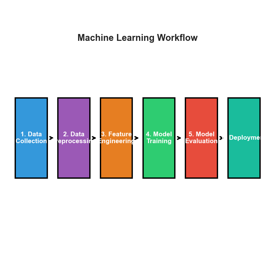
The ML Pipeline: From Data to Deployment

See visual diagram in lecture materials

Key Insight

ML is iterative! Model performance informs feature engineering, data collection, etc.

Data Preprocessing: Cleaning & Scaling

            Data Cleaning
            Missing values: Imputation or deletion
Outliers: Detect and handle
Duplicates: Remove
Noise: Filter/smooth

        

Feature Scaling

Z-score: $z = \frac{x - \mu}{\sigma}$

Min-Max: $x' = \frac{x - \min}{\max - \min}$

Robust: Uses median/IQR

Why Scale?

Many algorithms (SVM, KNN, gradient descent) are sensitive to feature scales!

Feature Engineering & Train/Test Split

            Feature Engineering
            Polynomial features: $x_1 x_2$, $x^2$
One-hot encoding
Date/time extraction
Text vectorization (TF-IDF)

        

Train/Test Split

Common: 80/20 or 70/30
Cross-validation (k-fold)
Time series: temporal split

Rule: Never train on test data!

Python Example

from sklearn.preprocessing import StandardScaler
from sklearn.impute import SimpleImputer

imputer = SimpleImputer(strategy='mean')
scaler = StandardScaler()
X_clean = scaler.fit_transform(imputer.fit_transform(X))

Model Selection \& Training

Choosing a ModelConsider:
Problem type: Regression, classification, etc.
Data size: Deep learning needs more data
Interpretability: Linear models vs black boxes
Training time: Real-time vs offline
Prediction speed: Production requirements

No Free Lunch TheoremTheorem: No single algorithm works best for all problems

Implication: Must try multiple approaches and validate empirically

Start Simple!

Simple baseline (mean, majority class)
Linear model
More complex models
Ensemble methods

Training ProcessOptimization: Minimize loss function
$$\theta^* = \arg\min_\theta \mathcal{L}(\theta; \mathcal{D})$$

Common Optimizers:
Gradient Descent
Stochastic Gradient Descent (SGD)
Adam (adaptive learning rate)
RMSprop

Hyperparameter TuningHyperparameters: Set before training
Learning rate, regularization strength
Number of layers, hidden units
Tree depth, number of trees


Search Methods:
Grid search
Random search
Bayesian optimization

Model Evaluation Metrics

Regression MetricsMean Squared Error (MSE):
$$\text{MSE} = \frac{1}{n}\sum_{i=1}^n (y_i - \hat{y}_i)^2$$

Root MSE (RMSE):
$$\text{RMSE} = \sqrt{\text{MSE}}$$

Mean Absolute Error (MAE):
$$\text{MAE} = \frac{1}{n}\sum_{i=1}^n |y_i - \hat{y}_i|$$

R-squared (coefficient of determination):
$$R^2 = 1 - \frac{\sum_i (y_i - \hat{y}_i)^2}{\sum_i (y_i - \bar{y})^2}$$

Range: $(-\infty, 1]$, closer to 1 is better

Classification MetricsAccuracy:
$$\text{Acc} = \frac{\text{correct predictions}}{\text{total predictions}}$$

Precision (positive predictive value):
$$\text{Prec} = \frac{TP}{TP + FP}$$

Recall (sensitivity, true positive rate):
$$\text{Rec} = \frac{TP}{TP + FN}$$

F1-Score (harmonic mean):
$$F_1 = 2 \cdot \frac{\text{Prec} \cdot \text{Rec}}{\text{Prec} + \text{Rec}}$$

ROC-AUC: Area under ROC curve

Important

Choose metrics appropriate to your problem! Accuracy misleading for imbalanced data.

When to Use Each Metric

MetricUse WhenAvoid When

AccuracyBalanced classesImbalanced data
PrecisionFalse positives costlyNeed recall
RecallFalse negatives costlyNeed precision
F1-ScoreBalance precision/recallClear preference
RMSEPenalize large errorsRobust to outliers
MAEAll errors equalLarge errors matter

Metric	Use When	Avoid When
Accuracy	Balanced classes	Imbalanced data
Precision	False positives costly	Need recall
Recall	False negatives costly	Need precision
F1-Score	Balance precision/recall	Clear preference
RMSE	Penalize large errors	Robust to outliers
MAE	All errors equal	Large errors matter

Bias-Variance Tradeoff

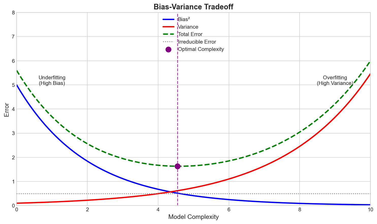
            Error Decomposition
            $$\text{Error} = \text{Bias}^2 + \text{Variance} + \text{Noise}$$
            Bias: Error from wrong assumptions
Variance: Sensitivity to training set
Noise: Irreducible error

        

The Tradeoff

Simple models: High bias, low variance
Complex models: Low bias, high variance

Underfitting vs Overfitting

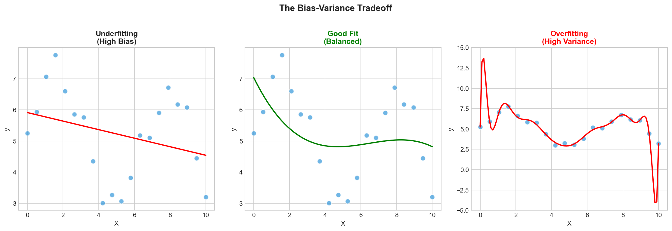
Overfitting Example — Underfitting vs Good Fit vs Overfitting

Underfitting

High train & test error

Fix:

More features
Complex model
Less regularization

Overfitting

Low train, high test error

Fix:

More data
Regularization
Simpler model

Regularization Techniques

L2 Regularization (Ridge)Modified objective:
$$\min_\theta \mathcal{L}(\theta) + \lambda \|\theta\|_2^2$$

where $\lambda > 0$ is regularization strength

Effect:
Penalizes large weights
Shrinks coefficients toward zero
Improves generalization
Handles multicollinearity


Closed-form solution (linear regression):
$$\hat{\theta} = (\mathbf{X}^T\mathbf{X} + \lambda \mathbf{I})^{-1}\mathbf{X}^T\mathbf{y}$$

L1 Regularization (Lasso)Modified objective:
$$\min_\theta \mathcal{L}(\theta) + \lambda \|\theta\|_1$$

Effect:
Sparse solutions (some $\theta_i = 0$)
Automatic feature selection
More aggressive than L2


No closed-form: Use iterative methods

Elastic Net

Combines L1 and L2: $$\min_\theta \mathcal{L}(\theta) + \lambda_1 \|\theta\|_1 + \lambda_2 \|\theta\|_2^2$$ Benefits:

Sparsity from L1
Stability from L2
Best of both worlds

Python Example: Ridge and Lasso

from sklearn.linear_model import Ridge, Lasso, ElasticNet

# Ridge (L2 regularization)
ridge = Ridge(alpha=1.0)
ridge.fit(X_train, y_train)

# Lasso (L1 regularization)
lasso = Lasso(alpha=0.1)
lasso.fit(X_train, y_train)

# Elastic Net (L1 + L2)
elastic = ElasticNet(alpha=0.1, l1_ratio=0.5)
elastic.fit(X_train, y_train)

# Lasso creates sparse solutions (feature selection)
print(f"Non-zero coefficients: {sum(lasso.coef_ != 0)}")

The Curse of Dimensionality

Problem StatementAs dimensionality $d$ increases:
Volume grows exponentially: $V \propto r^d$
Data becomes sparse: Points far apart
Distance metrics break down: All points equidistant
Overfitting risk increases: More parameters to fit

Mathematical InsightIn high dimensions, volume concentrated in corners:

$$\frac{V_{\text{corners}}}{V_{\text{total}}} = 1 - \left(1 - \frac{1}{2^d}\right)^{2^d} \approx 1 - e^{-1}$$

For unit hypercube, most volume is near edges!

Data Requirements

To maintain density, need $n \propto c^d$ samples where $c > 1$

Solutions1. Dimensionality Reduction
PCA, t-SNE, UMAP
Feature selection


2. Feature Selection
Filter methods (correlation)
Wrapper methods (RFE)
Embedded (Lasso, trees)


3. Regularization
L1/L2 penalties
Early stopping


4. Collect More Data
Exponentially more needed
Often impractical

Rule of Thumb

$n \geq 10 \cdot d$ for reliable models

CMSC 173 Course Topics

Core FoundationsI. Overview (Today!)
Learning paradigms
Applications


II. Parameter Estimation
Method of Moments
Maximum Likelihood Estimation


III. Regression
Linear Regression
Lasso & Ridge
Cubic Splines


IV. Model Selection
Bias-Variance Decomposition
Cross-Validation
Regularization

Advanced MethodsV. Classification
Logistic Regression, Naïve Bayes
KNN, Decision Trees


VI. Kernel Methods
Support Vector Machines
Kernel trick


VII. Dimensionality Reduction
Principal Component Analysis


VIII. Neural Networks
Feedforward Networks
CNNs, Transformers
Generative Models


IX. Clustering
K-Means, Hierarchical
Gaussian Mixture Models

Learning Resources

Recommended TextbooksPrimary:
Murphy, K. P. (2022). Probabilistic Machine Learning: An Introduction. MIT Press.
Bishop, C. M. (2006). Pattern Recognition and Machine Learning. Springer.


Supplementary:
Hastie et al. (2009). The Elements of Statistical Learning. Springer.
Goodfellow et al. (2016). Deep Learning. MIT Press.

Online ResourcesScikit-learn documentation
PyTorch/TensorFlow tutorials
Coursera ML courses (Andrew Ng)
Stanford CS229 lecture notes
ArXiv.org for research papers

Tools We'll Use

Python 3.8+
NumPy, Pandas, Matplotlib
Scikit-learn
Jupyter Notebooks
PyTorch (for deep learning)

Installation

Ensure you have Python and required packages installed before next session!

Best Practices in Machine Learning

"The best way to predict the future is to invent it." --- Alan Kay

Development Workflow1. Start with baseline
Simple model first
Establish minimum performance


2. Iterate systematically
Change one thing at a time
Track experiments
Version control (Git)


3. Validate rigorously
Cross-validation
Hold-out test set
Statistical significance


4. Document everything
Assumptions
Hyperparameters
Results

Common Pitfalls to AvoidData leakage: Test data in training
Ignoring class imbalance
Not checking for overfitting
Using wrong metrics
Not scaling features
Forgetting randomness: Set seeds!
Over-engineering: Keep it simple

Reproducibility

Essential for science:

Set random seeds
Document dependencies
Share code & data (when possible)
Report all hyperparameters

Ethics \& Responsible AI

"With great power comes great responsibility." --- Stan Lee (adapted from Voltaire)

Ethical ConsiderationsBias & Fairness:
Training data may contain biases
Models can amplify discrimination
Ensure fairness across groups


Privacy:
Protect sensitive information
Anonymization techniques
Comply with regulations (GDPR)


Transparency:
Explainable AI (XAI)
Interpretable models
Document limitations


Safety & Security:
Adversarial robustness
Prevent misuse
Validate thoroughly

Societal ImpactPositive:
Healthcare improvements
Scientific discoveries
Accessibility tools
Environmental monitoring


Concerns:
Job displacement
Deepfakes & misinformation
Surveillance
Autonomous weapons

Our Responsibility

As ML practitioners, we must:

Consider ethical implications
Design inclusive systems
Communicate limitations
Prioritize societal benefit

Key Takeaways

What We Covered TodayDefinition of Machine Learning: Learning from data to improve performance
Supervised Learning: Regression & classification with labeled data
Unsupervised Learning: Clustering & dimensionality reduction
Semi-Supervised Learning: Leveraging both labeled & unlabeled data
Reinforcement Learning: Learning through interaction & rewards
ML Pipeline: From data collection to deployment
Key Challenges: Bias-variance tradeoff, overfitting, curse of dimensionality
Best Practices: Systematic development, validation, ethics

Next Lecture

Parameter Estimation: Method of Moments & Maximum Likelihood Estimation

Prepare for Next Session

Required ReadingMurphy (2022):
Chapter 4: Statistics (4.1-4.3)
Chapter 5: Decision Theory (5.1-5.2)


Bishop (2006):
Chapter 1: Introduction (1.1-1.5)
Chapter 2: Probability (2.1-2.3)

Practice Problems

Review probability theory
Linear algebra refresher
Set up Python environment
Install required packages

Questions to PonderWhen would you choose supervised vs unsupervised learning?
How do you decide on train/test split ratio?
What metrics are appropriate for imbalanced datasets?
How can we detect overfitting early?
What are ethical concerns in your domain of interest?