Probability &
Statistical Foundations
CMSC 178DA - Week 02
Noel Jeffrey Pinton
Department of Computer Science
University of the Philippines Cebu
Learning Objectives
Lecture 3: Probability Review
- Review fundamental probability concepts
- Apply Bayes' theorem to real-world problems
- Understand common probability distributions
- Connect probability to data analytics applications
Why Probability Matters
Probability: A number between 0 and 1 that measures the likelihood of an event occurring. It quantifies uncertainty in data and predictions.
Uncertainty is Everywhere
- Will this customer churn?
- Is this transaction fraudulent?
- Will it rain tomorrow?
- Is this drug effective?
Probability in Data Analytics
Probability is the foundation for everything we'll learn
Powers These Methods
- Hypothesis testing — Is this effect real?
- Machine learning — Predict outcomes
- Statistical inference — Draw conclusions
This Week's Roadmap
- Probability rules & Bayes' theorem
- Distributions & CLT
- Hypothesis testing & confidence intervals
Set Operations in Probability
Before we combine probabilities, let's review set notation
A ∪ B (Union)
A or B (or both)
A ∩ B (Intersection)
A and B (both)
A' (Complement)
not A
Sample Space (S): The set of all possible outcomes · Event: A subset of outcomes we care about
Basic Probability Rules
S = sample space · A, B = events · A∩B = intersection
Fundamental Rules
$$P(S) = 1$$
$$P(A') = 1 - P(A)$$
$$P(A \cup B) = P(A) + P(B) - P(A \cap B)$$
Every probability must be between 0 and 1: $0 \leq P(A) \leq 1$
Reading P(A|B) Notation
Before we use this notation, let's understand what it means
$$P(A \mid B)$$
$P(A|B)$
"Probability of A"
$\mid$
"given that"
$B$
"B already happened"
Example: P(Rain | Cloudy) = "If it's cloudy, what's the chance of rain?"
We're not asking about all days — only cloudy days
Conditional Probability
Conditional Probability: The probability of event A occurring, given that event B has already occurred. It measures how B affects our belief about A.
$$P(A|B) = \frac{P(A \cap B)}{P(B)}$$
GCash User Example
- 57% of GCash users are women
- Assume: 70% of women users use GCash for bills payment
- $P(\text{Bills} | \text{Women}) = 0.70$
What's the probability a random user pays bills AND is a woman?
$P(\text{Bills} \cap \text{Women}) = 0.70 \times 0.57 = 0.40$
Source: GCash Statistics 2024 · 70% assumption for illustration
Independence
Definition: A and B are independent if:
$$P(A \cap B) = P(A) \times P(B)$$
Independent Events
- Coin flip 1 vs Coin flip 2
- Rain in Cebu vs Rain in Manila
Dependent Events
- Rain today vs Rain tomorrow
- Age vs Income
Caution: Independence is often assumed but rarely verified!
Introducing Bayes' Theorem
Thomas Bayes (1701-1761)
English minister and mathematician who asked: "How should we update our beliefs when we see new evidence?"
- Published posthumously in 1763
- Rediscovered by Pierre-Simon Laplace
- Now one of the most-used formulas in all of statistics
Why It Matters Today
- Spam filters (Gmail uses it)
- Medical diagnosis
- Search engines & recommendations
- Self-driving cars
- Machine learning & AI
Bayes' Intuition: Updating Beliefs
Bayes gives us a systematic way to update what we believe
Prior Belief
What you believed before seeing data
New Evidence
Data you just observed
Posterior
Your updated belief
Everyday example: You hear thunder.
Before hearing it: 30% chance of rain → After hearing thunder: 80% chance of rain
That update is Bayes' Theorem in action.
Bayes' Theorem
$$P(A|B) = \frac{P(B|A) \cdot P(A)}{P(B)}$$
| Term | Name |
|---|---|
| $P(A|B)$ | Posterior |
| $P(B|A)$ | Likelihood |
| $P(A)$ | Prior |
| $P(B)$ | Evidence |
Key Insight:
Bayes' theorem lets us update our beliefs when we get new evidence.
Medical Testing Vocabulary
Before we apply Bayes' theorem, learn these key terms
| Term | Symbol | What It Means | Example |
|---|---|---|---|
| Prevalence | $P(D)$ | % of population with disease | 1% have diabetes |
| Sensitivity | $P(+|D)$ | % of sick people who test positive | 95% detection rate |
| Specificity | $P(-|\neg D)$ | % of healthy people who test negative | 90% correctly cleared |
Key Question: If someone tests positive, what's the actual probability they have the disease?
(Hint: It's NOT the sensitivity!)
Bayes' Example: Medical Testing
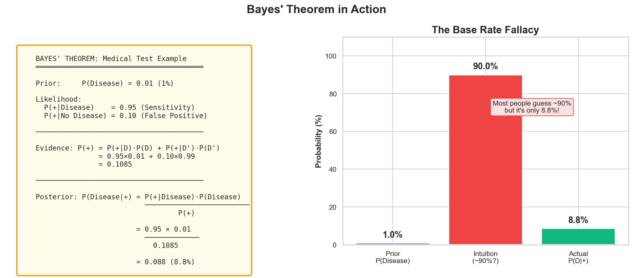
Most people intuitively guess ~90%. The actual probability is only 8.8%!
Bayes' Calculation
Step 1: Total Probability of Positive
$$P(+) = P(+|D) \cdot P(D) + P(+|\neg D) \cdot P(\neg D)$$
$= 0.95 \times 0.01 + 0.10 \times 0.99 = \mathbf{0.1085}$
Step 2: Apply Bayes' Theorem
$$P(D|+) = \frac{P(+|D) \cdot P(D)}{P(+)}$$
$= \frac{0.95 \times 0.01}{0.1085} = \mathbf{0.088}$
Result: Only 8.8% chance of disease despite positive test!
Random Variables
Random Variable: A variable whose value is determined by the outcome of a random process. It maps outcomes to numerical values.
Discrete
Countable outcomes
- Number of transactions per day
- Customer complaints count
- Number of app downloads
Continuous
Infinite possible values
- Transaction amount
- Customer lifetime value
- Response time (seconds)
Greek Letter Cheat Sheet
Statistics uses Greek letters as shorthand — here's what they mean
| Symbol | Name | Meaning | Example |
|---|---|---|---|
| μ | mu (mew) | Population mean (true average) | μ = 170 cm (avg height) |
| σ | sigma | Standard deviation (spread) | σ = 10 cm |
| $\bar{x}$ | x-bar | Sample mean (measured average) | $\bar{x}$ = 168 cm |
| Σ | Sigma (big) | Summation ("add up all...") | Σx = sum of all values |
μ and σ describe the population (what we want to know) · $\bar{x}$ comes from our sample (what we can measure)
Expected Value & Variance
Expected Value (Mean): The long-run average of a random variable
Variance: How spread out values are from the mean
Expected Value
Discrete: $E[X] = \sum x \cdot P(X=x)$
Continuous: $E[X] = \int x \cdot f(x) \, dx$
Variance
$$Var(X) = E[(X - \mu)^2]$$
Shortcut: $Var(X) = E[X^2] - (E[X])^2$
Standard Deviation: $\sigma = \sqrt{Var(X)}$ — same units as the data
Example: Is Lotto Worth It?
Let's calculate the expected value of a ₱20 lotto ticket
| Prize | Probability | × Value |
|---|---|---|
| ₱0 (lose) | 0.99 | ₱0.00 |
| ₱50 (minor) | 0.008 | ₱0.40 |
| ₱500 | 0.0019 | ₱0.95 |
| ₱10M (jackpot) | 0.0001 | ₱1,000 |
$E[X] = \sum x \cdot P(X=x) = 0 + 0.40 + 0.95 + 1000$
E[X] ≈ ₱1,001.35
Wait... that seems profitable? 🤔
Lotto: The Reality Check
Actual jackpot probability: 1 in 40,475,358
That makes E[X] ≈ ₱1.24, not ₱1,001
You pay ₱20, expect ₱1.24 back
→ Lose ₱18.76 on average per ticket!
Lesson: Expected value reveals hidden costs that intuition misses
Source: PCSO Ultra Lotto 6/58 (official odds)
What is a Probability Distribution?
A probability distribution describes how likely each possible outcome is
Think of it as a "shape of uncertainty"
Discrete Distribution
Countable outcomes (dice sum)
Binomial, Poisson
Continuous Distribution
Infinite values (heights)
Normal, Exponential
Different phenomena follow different distributions — choosing the right one is key!
Why the Right Distribution Matters
Choosing the wrong distribution leads to wrong conclusions
Correct Choices
- Customer wait times → Exponential
- Exam scores → Normal
- Defect counts → Poisson
- Pass/fail outcomes → Binomial
Wrong Choices
- Normal for count data → can predict negative counts!
- Normal for income data → misses the long right tail
- Binomial when trials aren't independent → wrong variance
Always check your data's shape before choosing a distribution
Common Probability Distributions
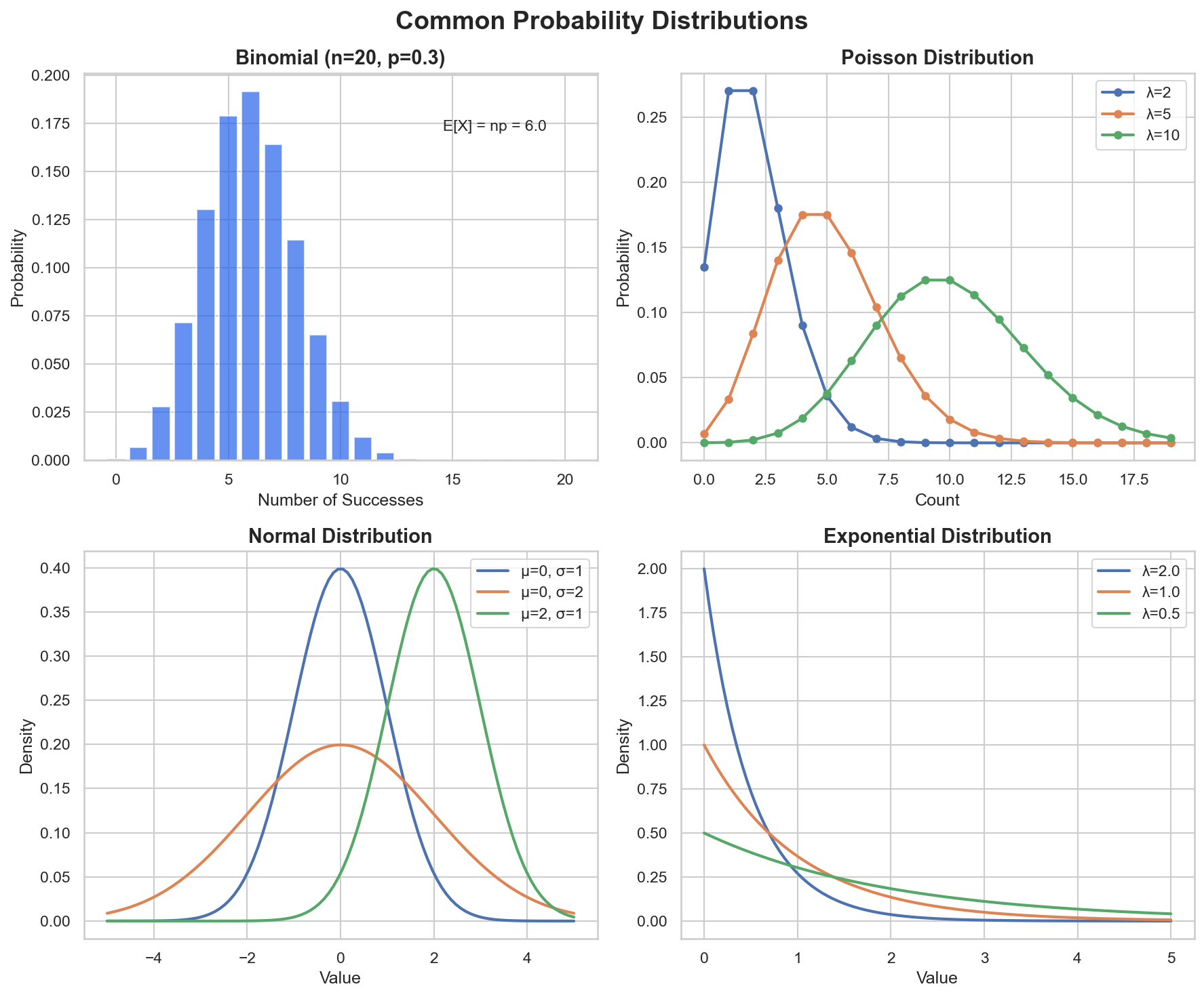
Different distributions model different types of data: counts, rates, continuous measurements
When to Use: Binomial
Models the number of successes in a fixed number of independent yes/no trials
3 Requirements
- Fixed number of trials ($n$)
- Each trial: success or failure only
- Same probability ($p$) each trial, trials independent
Real Examples
- Coin flips: heads in 10 tosses
- MCQ guessing: correct in 20 questions
- Defective items in a batch of 100
- Free throw success in 15 attempts
Binomial Distribution
When to use: Counting successes in fixed number of trials
$$P(X=k) = \binom{n}{k} p^k (1-p)^{n-k}$$
Example: Loan Applications
10 loan applications, 30% approval rate. P(exactly 5 approvals)?
from scipy.stats import binom

# P(exactly 5 approvals out of 10, approval rate 30%)
prob = binom.pmf(5, n=10, p=0.3)
print(f"P(X=5) = {prob:.4f}")  # Output: 0.1029
When to Use: Poisson
Models the count of events in a fixed interval of time or space, when events occur independently at a constant average rate
3 Requirements
- Events occur independently
- Average rate ($\lambda$) is constant
- Two events cannot occur at exactly the same instant
Real Examples
- Calls to a hotline per hour
- Typos per page of a book
- Jeepney arrivals per 10 minutes
- Website visitors per minute
Poisson Distribution
When to use: Rare events in fixed time/space
$$P(X=k) = \frac{\lambda^k e^{-\lambda}}{k!}$$
Example: Website Traffic
Website receives avg 20 visits/hour. P(exactly 25 visits)?
from scipy.stats import poisson

# P(exactly 25 visits, avg rate 20/hour)
prob = poisson.pmf(25, mu=20)
print(f"P(X=25) = {prob:.4f}")  # Output: 0.0446
The Normal Distribution
The most important distribution in statistics
Many natural phenomena follow this bell-shaped curve when sample sizes are large enough
Also called the Gaussian distribution, after Carl Friedrich Gauss (1777-1855)
Why It's So Important
- The Central Limit Theorem guarantees sample means are approximately Normal
- Required assumption for many statistical tests (t-test, ANOVA, regression)
- Heights, exam scores, measurement errors all follow it naturally
Normal Distribution
Normal (Gaussian) Distribution: A symmetric, bell-shaped distribution defined by mean ($\mu$) and standard deviation ($\sigma$).
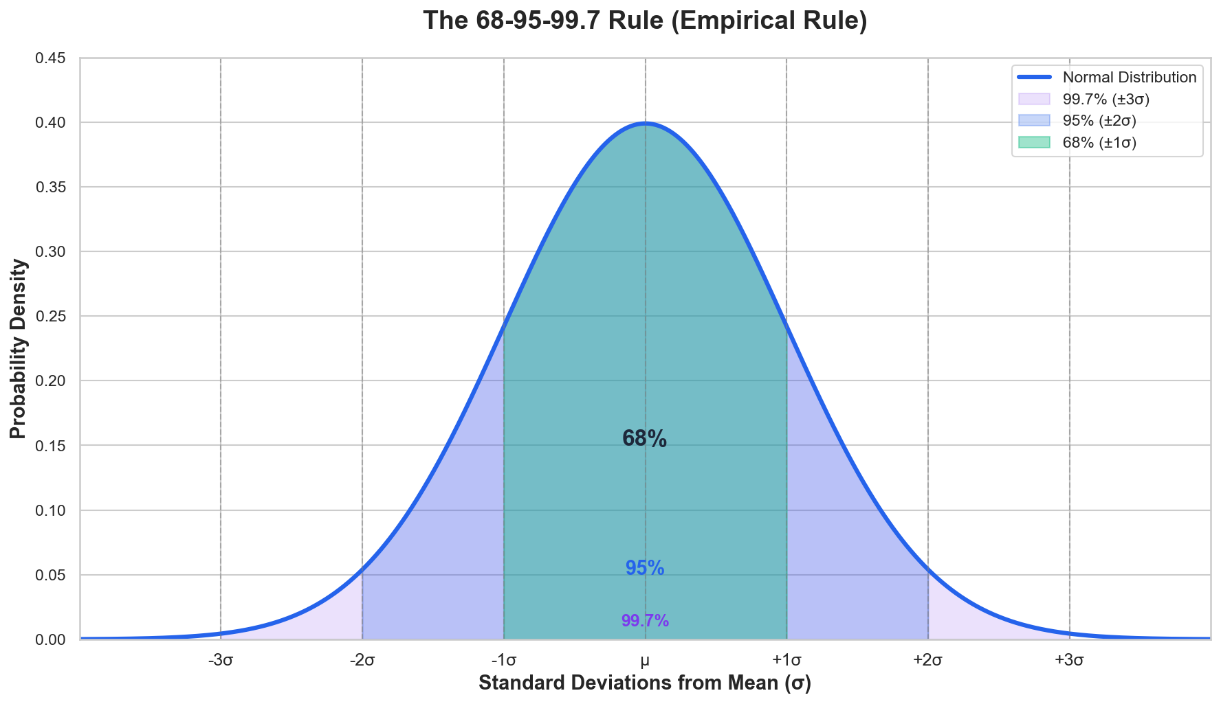
The 68-95-99.7 Rule
- 68% within $\pm 1\sigma$
- 95% within $\pm 2\sigma$
- 99.7% within $\pm 3\sigma$
This rule is used to identify outliers and assess data normality
Central Limit Theorem
The Most Important Theorem in Statistics
"The sampling distribution of the mean approaches normal as sample size increases, regardless of population distribution."
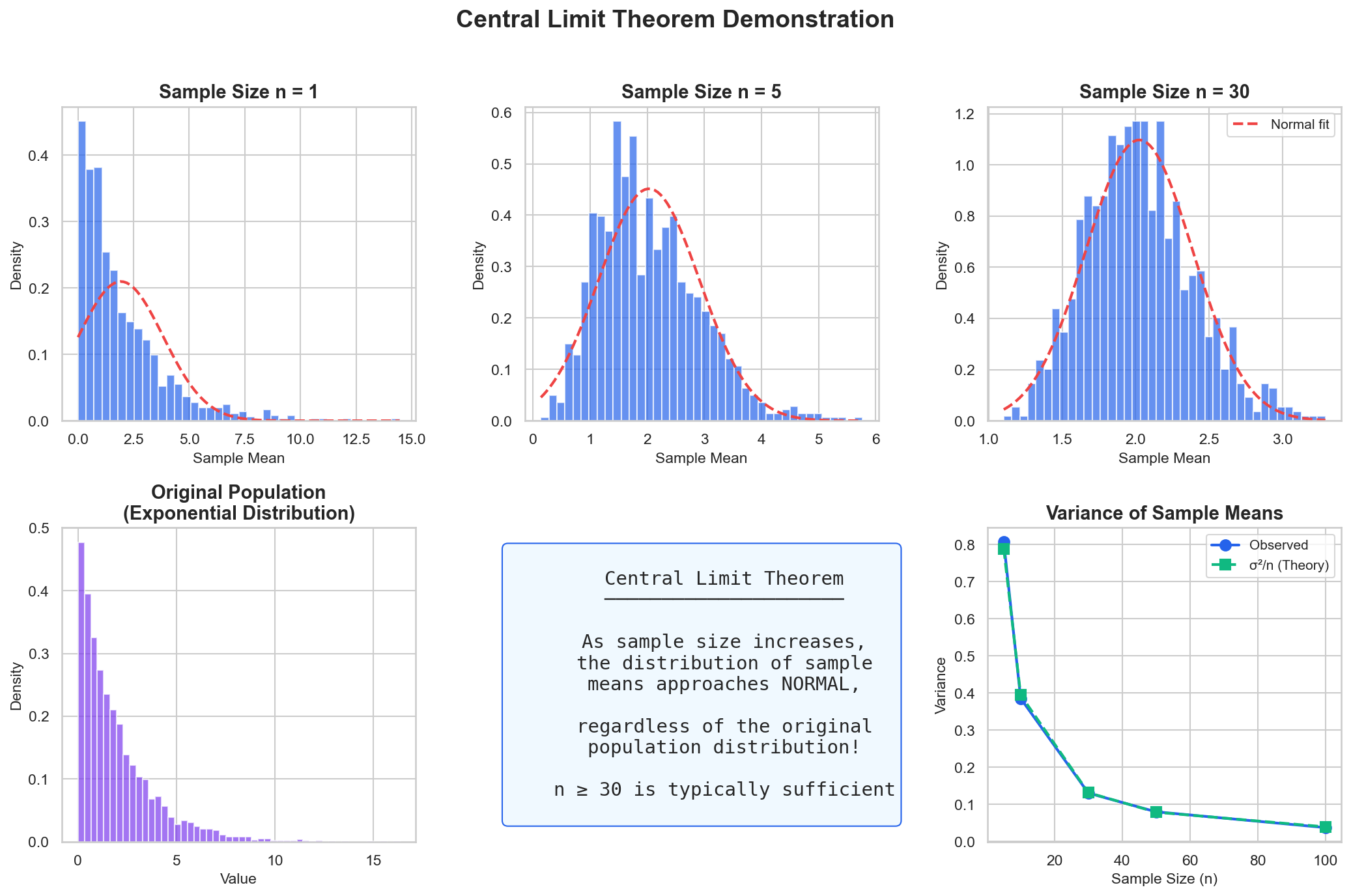
As sample size increases: exponential population → normal sample means
CLT Demonstration
# Exponential population (skewed, not normal!)
population = np.random.exponential(scale=2, size=100000)

# Take 1000 samples, compute means → Normal!
sample_means = [np.random.choice(population, 30).mean()
                for _ in range(1000)]

plt.hist(sample_means, bins=30)
Skewed exponential population → Normal distribution of sample means (n=30)
Wrong Distribution = Wrong Conclusions
Choosing the wrong distribution leads to misleading results
Example 1: Income Data
If you assume income is Normal (symmetric), you will:
- Underestimate the number of very high earners
- Overestimate the "average" person
Better: Log-normal distribution (right-skewed)
Example 2: Rare Events
If you model server crashes with Normal, you might:
- Predict "negative crashes" (impossible!)
- Underestimate extreme events
Better: Poisson (handles count data correctly)
Always: (1) Visualize your data first (2) Check skewness and shape (3) Run a normality test if using Normal
Real-World: Fraud Detection
BPI Credit Card Fraud Detection
Problem:
- Transaction amounts vary widely
- Need to flag unusual transactions
- Balance false positives vs fraud
Solution:
- Model with log-normal distribution
- Flag transactions > 3σ from mean
- Bayes to update fraud probability
Source: BSP Payment Systems Reports · Approach based on industry fraud detection practices
In-Class Exercise
GCash Fraud Detection with Bayes
Given:
- 5% of GCash transactions are flagged for review
- Of flagged transactions, 20% are actually fraudulent
- Of non-flagged transactions, 0.1% are fraudulent
Calculate:
- What is P(Fraudulent)?
- What is P(Flagged | Fraudulent)?
- If a transaction is fraudulent, what's the probability it was flagged?
Hypothetical rates for illustration
Exercise Answer
1. P(Fraudulent)
$P(F) = P(F|Flag) \cdot P(Flag) + P(F|\neg Flag) \cdot P(\neg Flag)$
$= 0.20 \times 0.05 + 0.001 \times 0.95$
$= 0.01 + 0.00095 = \mathbf{0.01095}$
≈ 1.1% of transactions are fraudulent
2 & 3. P(Flagged | Fraudulent)
Using Bayes' Theorem:
$P(Flag|F) = \frac{P(F|Flag) \cdot P(Flag)}{P(F)}$
$= \frac{0.20 \times 0.05}{0.01095} = \frac{0.01}{0.01095}$
≈ 91.3% of fraud gets flagged
Insight: The system catches 91% of fraud, but most flagged transactions (80%) are false alarms!
Key Takeaways - Probability
- Probability quantifies uncertainty in data and predictions
- Bayes' theorem updates beliefs with new evidence
- Different distributions fit different data types
- Central Limit Theorem enables normal-based inference
- These concepts underpin all statistical analysis
Lecture 4
Statistical Inference Essentials
Learning Objectives
Lecture 4: Statistical Inference
- Conduct and interpret hypothesis tests
- Construct and interpret confidence intervals
- Apply A/B testing framework
- Recognize limitations of p-values
From Data to Decisions
You survey 200 students at UP Cebu about their preferred payment app.
68% say GCash.
Can you conclude that 68% of ALL Filipino college students prefer GCash?
Statistical inference = using sample data to draw conclusions about a larger population, while quantifying our uncertainty
Sample vs Population
The fundamental distinction in statistics
Population (N)
Everyone you want to study
e.g., All 109M Filipinos
Sample (n)
Subset you actually measure
e.g., Survey of 1,000 people
Why sample? We can't measure everyone — so we measure a subset and infer about the whole
Population: PSA 2020 Census (109,035,343)
What is Statistical Inference?
Definition: Drawing conclusions about populations from samples
Estimation
What's the value?
- Point estimates
- Confidence intervals
Testing
Is there an effect?
- Hypothesis tests
- p-values
What is Hypothesis Testing?
A structured method for deciding whether observed data provides enough evidence to reject a claim about a population
Think of It Like a Court Trial
- Defendant = Your hypothesis
- "Innocent until proven guilty" = H₀ (null hypothesis)
- Prosecution's evidence = Your data
- Jury's standard of proof = Significance level (alpha)
- Verdict = Reject or fail to reject H₀
Just like a jury needs "beyond reasonable doubt," we need a p-value below alpha to reject H₀
The Logic of Hypothesis Testing
Hypotheses
α level
Calculate
p-value
Decision
Null vs Alternative Hypothesis
Null Hypothesis (H₀)
Status quo, no effect
- "There is no difference"
- "The parameter equals X"
- "The treatment has no effect"
Alternative Hypothesis (H₁)
What we're testing for
- "There is a difference"
- "The parameter ≠ X"
- "The treatment has an effect"
We never "prove" H₀ - we either reject it or fail to reject it
Types of Errors in Hypothesis Testing
The Confusion Matrix of Statistical Decisions
| H₀ Actually True | H₀ Actually False | |
|---|---|---|
| Reject H₀ |
✗ Type I Error (α) False Positive |
✓ Correct True Positive (Power) |
| Fail to Reject H₀ |
✓ Correct True Negative |
✗ Type II Error (β) False Negative |
Statistical Power = 1 − β (ability to detect a true effect when it exists)
Remember It: The Pregnancy Test
H₀: "You are NOT pregnant"
Type I Error (False Positive)
Telling a man he's pregnant
Detecting something that doesn't exist
Cost: Unnecessary panic, wasted resources
Type II Error (False Negative)
Telling a pregnant woman she's not
Missing something that does exist
Cost: Delayed prenatal care, health risks
Type II errors are often more dangerous — you miss a real condition!
The p-value
Definition: Probability of observing data as extreme as ours, assuming H₀ is true
Interpretation
- Small p (< α): Evidence against H₀
- Large p: Insufficient evidence against H₀
Common α Levels
- 0.05 (most common)
- 0.01 (more stringent)
- 0.10 (exploratory)
Critical Value Tables
Before computers, statisticians looked up critical values in printed tables
t-Distribution (excerpt)
| df | α=0.10 | α=0.05 | α=0.01 |
|---|---|---|---|
| 5 | 2.015 | 2.571 | 4.032 |
| 10 | 1.812 | 2.228 | 3.169 |
| 15 | 1.753 | 2.131 | 2.947 |
| 20 | 1.725 | 2.086 | 2.845 |
| ∞ | 1.645 | 1.960 | 2.576 |
Two-tailed test
χ² Distribution (excerpt)
| df | α=0.10 | α=0.05 | α=0.01 |
|---|---|---|---|
| 1 | 2.706 | 3.841 | 6.635 |
| 2 | 4.605 | 5.991 | 9.210 |
| 3 | 6.251 | 7.815 | 11.345 |
| 4 | 7.779 | 9.488 | 13.277 |
| 5 | 9.236 | 11.070 | 15.086 |
Right-tailed test
How to use: If |your statistic| > critical value → reject H₀
Traditional vs Modern Approach
Traditional (Table Lookup)
- Calculate test statistic (t or χ²)
- Find degrees of freedom (df)
- Look up critical value in table
- Compare: |statistic| > critical?
Example: t = 2.5, df = 10 → critical = 2.228 → Reject
Modern (Python)
from scipy import stats
t_stat, p_value = stats.ttest_ind(group1, group2)
if p_value < 0.05:
    print("Reject H₀")
No tables needed — exact p-value computed!
Both methods give the same answer — Python just automates the lookup
p-value in Plain Language
Scenario: Testing if a Coin is Fair
You flip a coin 10 times and get 9 heads. Is it unfair?
H₀: Coin is fair (P = 0.5)
H₁: Coin is biased
You calculate: p = 0.02
What p = 0.02 means:
"If the coin WERE fair, there's only a 2% chance of getting 9+ heads"
Conclusion: Since 2% < 5% (our α), we reject H₀
The result is "too weird" to happen by chance → evidence of bias
How We Got p = 0.02
The coin flip uses the Binomial Distribution
By Hand (Binomial Formula)
P(X ≥ 9) = P(X=9) + P(X=10)
$P(X=k) = \binom{n}{k} p^k (1-p)^{n-k}$
$P(9) = 10 \times 0.000977$ · $P(10) = 0.000977$
= 0.0107 (one-tailed) → 0.02 (two-tailed)
With Python
from scipy.stats import binom
p_value = 1 - binom.cdf(8, n=10, p=0.5)
# One-tailed: 0.0107
p_two = 2 * p_value  # Two-tailed: 0.02
Two-tailed p ≈ 0.02 because we'd also reject if we got 9+ tails (equally extreme)
t-test: Comparing Means
t-test: A statistical test used to compare means and determine if the difference is statistically significant. Used when sample size is small or population standard deviation is unknown.
One-sample t-test
Compare sample mean to known value
$$t = \frac{\bar{x} - \mu_0}{s / \sqrt{n}}$$
Two-sample t-test
Compare two group means
$$t = \frac{\bar{x}_1 - \bar{x}_2}{\sqrt{s_p^2(1/n_1 + 1/n_2)}}$$
t-test Example: Grab Earnings
Question: Do Grab drivers in Cebu earn more than Manila?
cebu = [850, 920, 780, 900, 870, 950, 820, 890, 880, 910]
manila = [800, 850, 750, 820, 780, 830, 770, 810, 790, 840]

t_stat, p_value = ttest_ind(cebu, manila)
# Output: t=3.162, p=0.0055 → Significant!
Data simulated based on LTFRB fare structures (hypothetical for illustration)
How t = 3.162 Was Computed
Step-by-step calculation for two-sample t-test
Step 1: Means & Variances
$\bar{x}_{Cebu} = 877$ | $\bar{x}_{Manila} = 804$
$s^2_{Cebu} = 2290$ | $s^2_{Manila} = 1160$ | $n = 10$
Step 2: Pooled Variance
$s_p^2 = \frac{(n_1-1)s_1^2 + (n_2-1)s_2^2}{n_1 + n_2 - 2} = \frac{9(2290) + 9(1160)}{18} = 1725$
Step 3: Standard Error
$SE = \sqrt{s_p^2 \cdot (\frac{1}{n_1} + \frac{1}{n_2})} = \sqrt{1725 \cdot 0.2} = 18.57$
Step 4: t-statistic
$t = \frac{\bar{x}_1 - \bar{x}_2}{SE} = \frac{877 - 804}{18.57}$ = 3.93
df = 18 → Critical t at α=0.05 is 2.101 → 3.93 > 2.101 → Reject H₀
Chi-Square Test
Purpose: Test independence of categorical variables
$$\chi^2 = \sum \frac{(O - E)^2}{E}$$
Example: Is payment method independent of age?
| Cash | GCash | Card | |
|---|---|---|---|
| Under 30 | 50 | 120 | 30 |
| 30-50 | 80 | 90 | 50 |
| Over 50 | 100 | 40 | 60 |
Illustrative data based on BSP 2021 Financial Inclusion Survey trends (e-wallets most common among ages 15-49)
Chi-Square in Python
# Contingency table: rows=age groups, cols=payment methods
table = np.array([[50, 120, 30],   # Under 30
                   [80, 90, 50],    # 30-50
                   [100, 40, 60]])  # Over 50

chi2, p_value, dof, expected = chi2_contingency(table)
# Output: chi2=62.89, p < 0.0001 → NOT independent!
How χ² = 62.89 Was Computed
Compare Observed (O) vs Expected (E) counts
Step 1: Calculate Expected Values
$E = \frac{Row Total \times Col Total}{Grand Total}$
| Cash | GCash | Card | |
|---|---|---|---|
| Under 30 | E=46 | E=100 | E=56 |
| 30-50 | E=51 | E=110 | E=62 |
| Over 50 | E=46 | E=100 | E=56 |
Step 2: Sum (O-E)²/E
$\chi^2 = \sum \frac{(O - E)^2}{E}$
$= \frac{(50-46)^2}{46} + \frac{(120-100)^2}{100} + ...$
χ² = 62.89, df = 4
Critical χ² at df=4, α=0.05 is 9.488 → 62.89 >> 9.488 → Reject H₀
Introducing Confidence Intervals
A range of plausible values for an unknown population parameter, based on sample data
Everyday Analogy
"How long is your commute?"
You wouldn't say "exactly 47 minutes"
You'd say "usually between 40-55 minutes"
A confidence interval gives this kind of range for statistical estimates
Why not just report the average? Because a single number hides the uncertainty in your estimate.
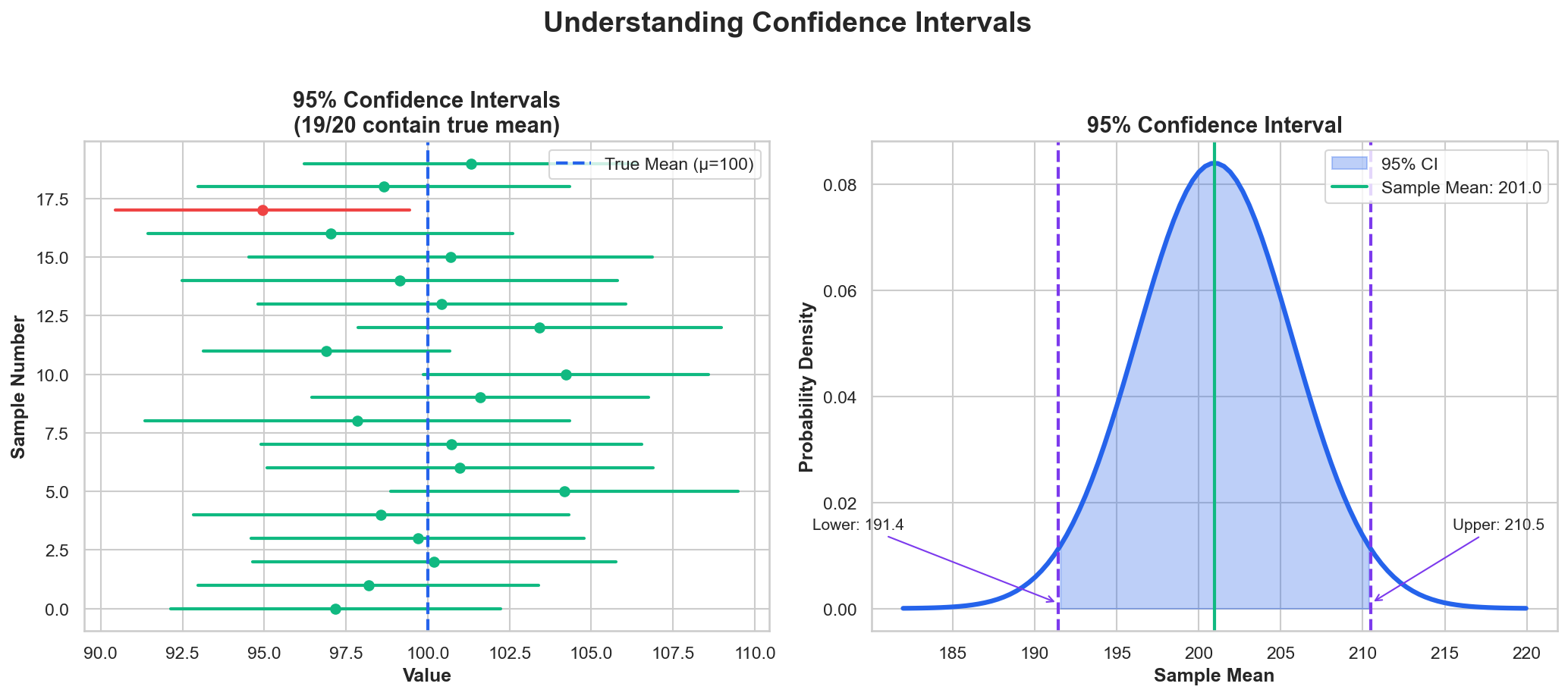
Confidence Intervals
Confidence Interval: Range likely to contain the true parameter
$$\bar{x} \pm t_{\alpha/2} \cdot \frac{s}{\sqrt{n}}$$
Correct: 95% of intervals contain the true mean
Wrong: "95% probability the mean is in this interval"
Confidence Interval Example
Estimate average GCash transaction amount
transactions = [150, 200, 180, 250, 175, 300, 220, 190,
                160, 280, 195, 210, 170, 240, 185]
mean = np.mean(transactions)
se = stats.sem(transactions)  # Standard error
ci = stats.t.interval(0.95, len(transactions)-1, mean, se)
# Output: mean=₱203.67, 95% CI: (₱178.42, ₱228.91)
Simulated data based on GCash transaction patterns
Introducing A/B Testing
A controlled experiment where you compare two versions (A and B) to see which performs better on a specific metric
You've Seen It Everywhere
- Netflix: Which thumbnail gets more clicks?
- Shopee: Which banner drives more sales?
- Facebook: Which feed algorithm keeps users longer?
- Google: Which search layout gets more engagement?
Why It Matters for Data Analysts
A/B testing is the gold standard for establishing causation, not just correlation.
It answers: "Did this change actually cause the improvement?"
A/B Testing Framework
Definition: Controlled experiment comparing two versions
Metric
Sample Size
Users
Experiment
Results
A/B Test Example: Lazada
Testing New Checkout Button Color
Control (A): Blue button
- 10,000 users
- 1,000 conversions (10%)
Treatment (B): Green button
- 10,000 users
- 1,100 conversions (11%)
Result: p = 0.04 → Green button wins!
Hypothetical scenario based on Lazada PH e-commerce patterns
Multiple Testing Problem
Problem: Running many tests increases false positives!
10 tests at α = 0.05:
$$P(\text{at least one false positive}) = 1 - 0.95^{10} = 40\%!$$
Bonferroni Correction
$$\alpha' = \frac{\alpha}{n}$$
For 10 tests: α' = 0.005
Other Solutions
- False Discovery Rate (FDR)
- Pre-registration
p-value Criticisms
Common Misinterpretations
- ❌ p-value is probability H₀ is true
- ❌ 1 - p = probability effect exists
- ❌ p < 0.05 means practically significant
Better Practice
- ✓ Report effect sizes
- ✓ Use confidence intervals
- ✓ Consider practical significance
Effect Size: Why It Matters
Effect Size: A standardized measure of the magnitude of a difference, independent of sample size. It tells you how big the effect is, not just whether it exists.
Statistical significance ≠ Practical significance
Large samples can make tiny effects "statistically significant"
Example: A drug reduces blood pressure by 0.5 mmHg (p < 0.001 with n=100,000) — statistically significant but clinically meaningless!
Cohen's d: Measuring Effect Size
$$d = \frac{\bar{x}_1 - \bar{x}_2}{s_{pooled}}$$
Difference in means ÷ Pooled standard deviation
| Interpretation | Cohen's d | Meaning |
|---|---|---|
| Small | 0.2 | Barely noticeable |
| Medium | 0.5 | Visible to careful observer |
| Large | 0.8 | Obvious to anyone |
Always report effect size alongside p-values!
In-Class Exercise
A/B Test Analysis
Data:
- Control: 500 users, 45 conversions (9%)
- Treatment: 500 users, 60 conversions (12%)
Tasks:
- Conduct a chi-square test for independence
- Calculate 95% CI for the difference in proportions
- Is a 3% lift practically significant for this business?
Exercise Answer
1. Chi-Square Test
| Conv | No Conv | |
|---|---|---|
| Control | 45 | 455 |
| Treatment | 60 | 440 |
$\chi^2 = 2.40$, df = 1
p ≈ 0.12 → Not significant at α=0.05
2. 95% CI for Difference
Difference = 12% − 9% = 3%
$SE = \sqrt{\frac{0.09 \times 0.91}{500} + \frac{0.12 \times 0.88}{500}} = 0.019$
95% CI = 3% ± 3.8%
CI: (−0.8%, 6.8%)
Contains 0 → not significant
3. Practical Significance: 3% lift = 15 extra conversions → ₱7,500 gain (if ₱500/conversion). Worth it if cost < ₱7,500!
Key Takeaways - Inference
- Hypothesis testing quantifies evidence against the null
- p-value is NOT the probability H₀ is true
- Confidence intervals provide range estimates
- A/B testing is gold standard for causal inference
- Effect size matters as much as statistical significance
Lab Preview
Lab 2: Statistical Testing in Python
- Part 1: t-tests on Philippine salary data
- Part 2: Chi-square on demographic data
- Part 3: Building an A/B test simulator
Datasets: PSA OpenSTAT Labor Force Survey, simulated GCash transaction patterns
Next Week
Week 3: Data Wrangling & Cleaning
Topics:
- Data collection methods
- SQL for data extraction
- Cleaning and transformation with pandas
- Handling missing values