CMSC 178DA | Week 7 · Session 1

Regression Analytics:
Explaining What Drives
the Numbers

From correlation to causal interpretation

Department of Computer Science

University of the Philippines Cebu

"Every coefficient tells a story about cause and effect."

"All models are wrong, but some are useful."

— George E.P. Box, 1976

This week: how to make regression useful for explaining and predicting in the Philippine context.

Agenda

Session 1 Objectives

Regression Fundamentals

The OLS equation, coefficient interpretation, and the meaning of “holding all else constant.”

Diagnostics & Assumptions

LINE assumptions, residual plots, VIF, and when to trust your model’s output.

Philippine Application

Regional poverty model using PSA data: literacy, GDP, and urbanization as predictors.

Part I

What Regression Answers

Regression in analytics is about explanation — not just prediction. The coefficients are the story.

Part I — What Regression Answers

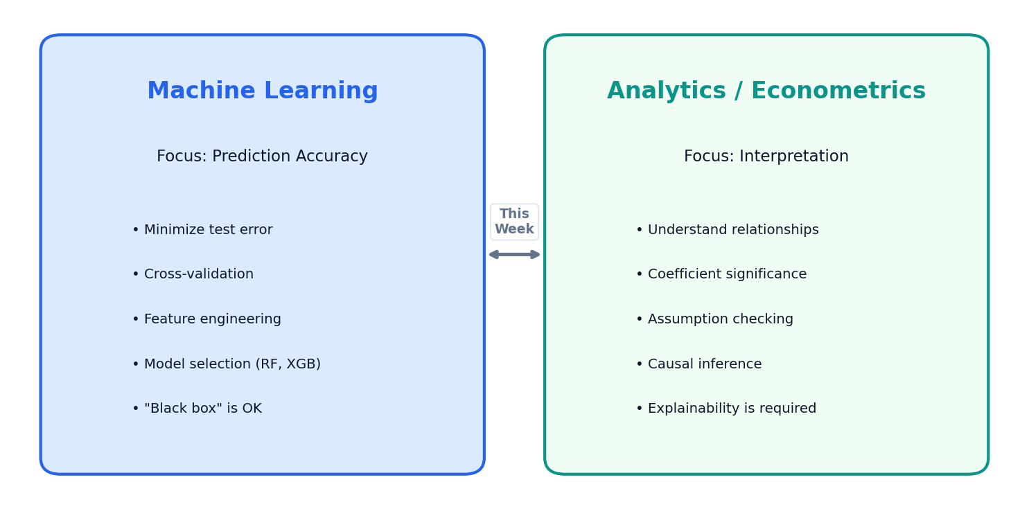
ML Predicts; Analytics Explains

ML prediction vs analytics explanation comparison
Part I — What Regression Answers

The Regression Equation Tells a Story

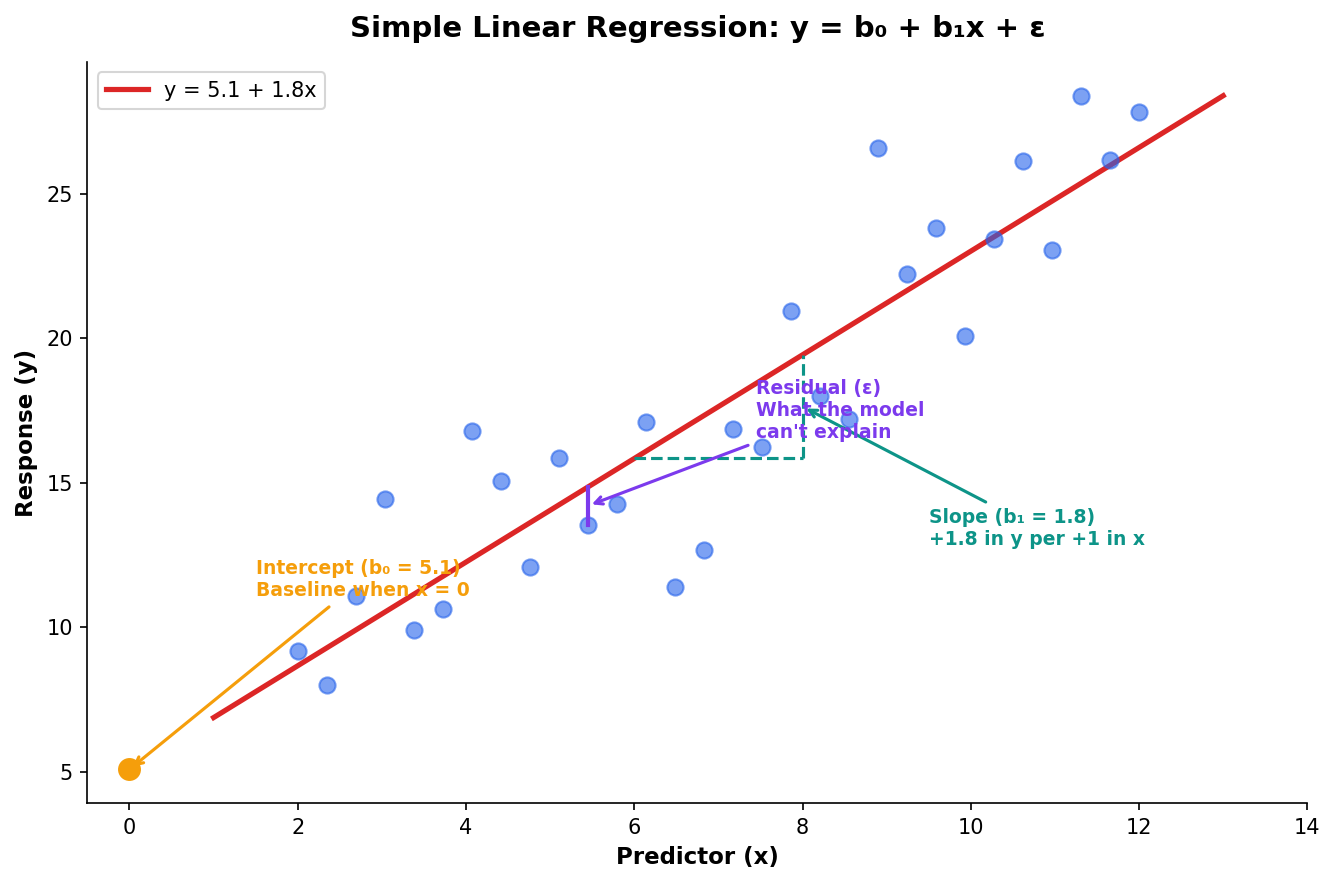
Every regression equation has three characters: the baseline (b₀), the effects (b₁, b₂…), and the unexplained (ε). Together they tell a story about what drives the outcome.

The Intercept (b₀)

The predicted value when all predictors are zero — often a theoretical baseline.

The Slope (b₁)

The change in y for a 1-unit increase in x, holding everything else constant.

Regression equation with labeled components
Part I — What Regression Answers

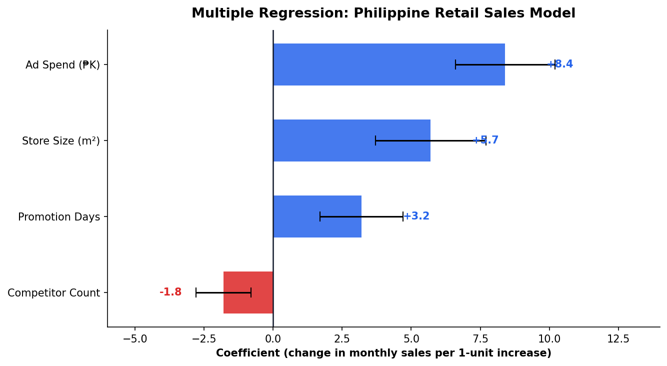
Each Coefficient Is a Ceteris Paribus Statement

Coefficient bar chart with confidence intervals
Part I — What Regression Answers

Interpreting Coefficients for Stakeholders

PredictorbTranslation
Ad Spend ₱K+8.4Each additional ₱1K in ads → ₱8.4K more sales
Store Size m²+5.7Larger stores sell more, all else equal
Promotion Days+3.2Each promo day adds ₱3.2K
Competitor Count−1.8Each nearby competitor costs ₱1.8K

Translation Rule

For every 1-unit increase in X, Y changes by b₁ units — holding all other variables constant.

What Stakeholders Want

They don’t want coefficients. They want: “Should we spend more on ads or open a bigger store?” Your regression answers this.

Part II

Trusting the Model

A regression is only as good as its assumptions. Visual diagnostics tell you when to trust — and when to stop.

Part II — Trusting the Model

LINE: Four Assumptions You Must Check

LINE assumptions: Linearity, Independence, Normality, Equal variance
Part II — Trusting the Model

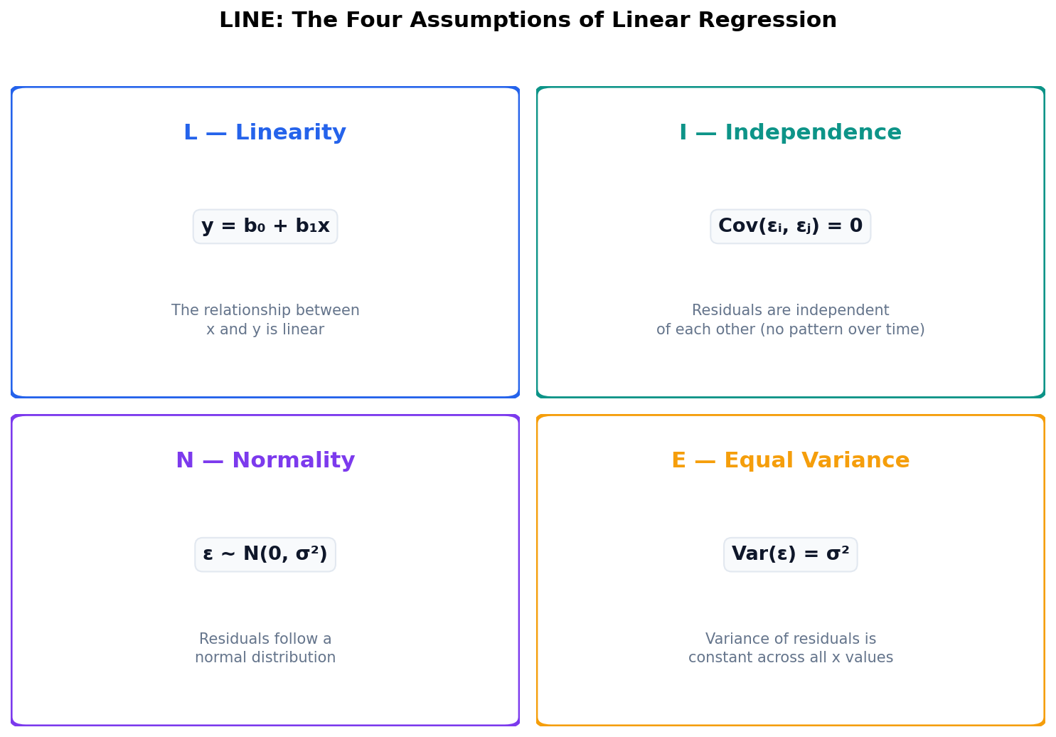
Residual Plots Reveal Hidden Problems

Residual plot and Q-Q plot diagnostics
Part II — Trusting the Model

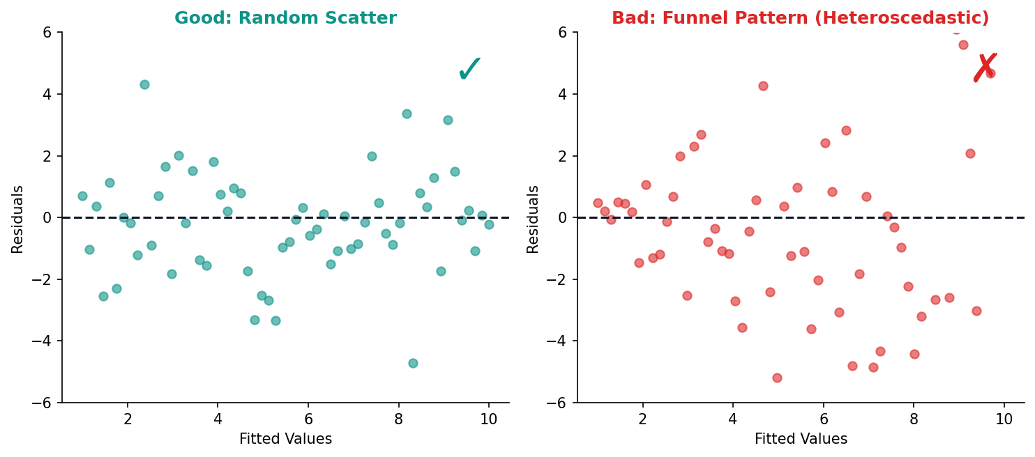
Good Residuals vs Bad Residuals

The residual plot is your first diagnostic check. Random scatter means the model’s assumptions hold. Patterns reveal specific problems.

✓ Good

Random scatter around zero — assumptions met.

× Bad

Funnel shape — variance increases with x (heteroscedasticity). Fix: log-transform y or use robust standard errors.

Good vs bad residual patterns side by side
Part II — Trusting the Model

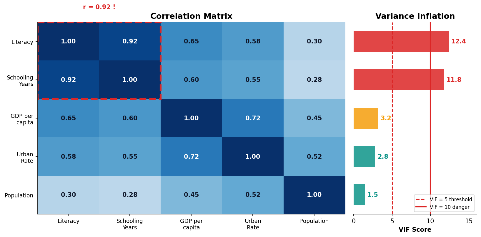
Multicollinearity Inflates Your Standard Errors

VIF heatmap showing multicollinearity among predictors
Part III

Model Evaluation & Application

R² tells you how much you explained. RMSE tells you how far off you are. Context tells you if the model is useful.

Part III — Model Evaluation & Application

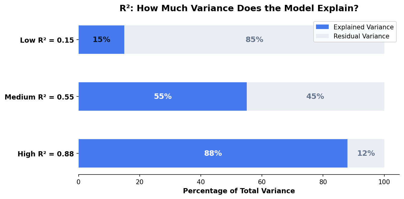
R² Measures Explained Variance

R-squared visual: explained vs unexplained variance
Part III — Model Evaluation & Application

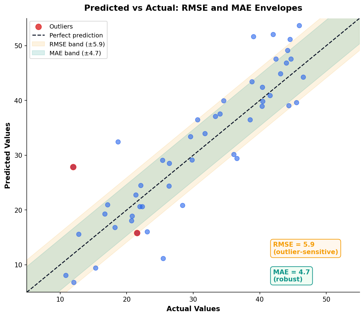
RMSE and MAE: Error in Units You Care About

Both measure prediction error in the same units as your outcome variable. RMSE penalizes large errors more heavily; MAE treats all errors equally.

MetricStrengthWeakness
RMSESensitive to outliersPenalizes big misses
MAERobust to outliersIgnores error magnitude

Practical Rule

Report both. If RMSE >> MAE, you have outlier predictions that need investigation.

RMSE vs MAE comparison on sample predictions
Part III — Model Evaluation & Application

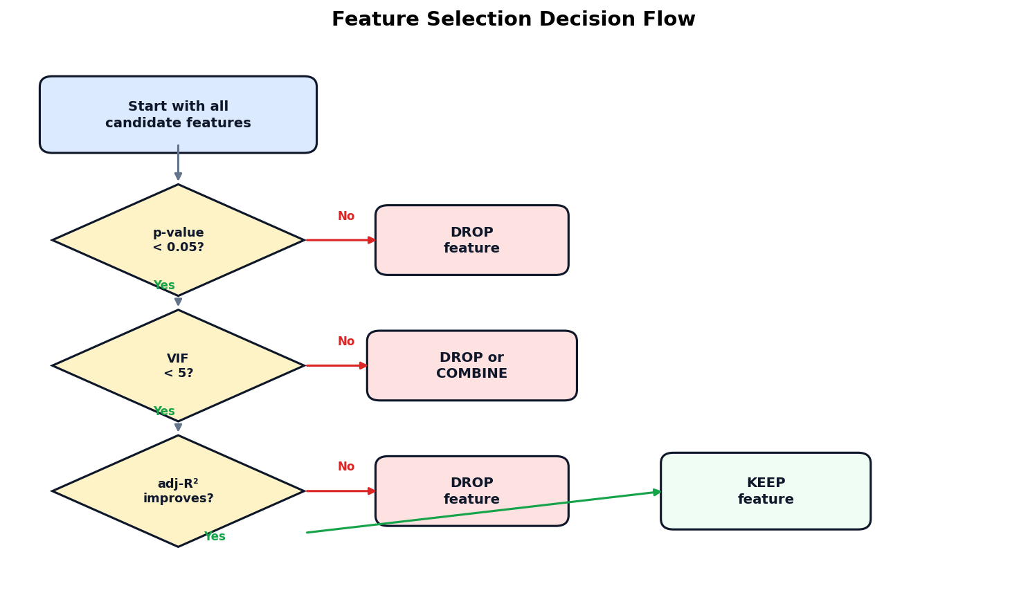
Feature Selection: Which Predictors Earn Their Place?

Feature selection decision flowchart
Part III — Model Evaluation & Application

Philippine Regional Poverty: A Regression Case Study

Scatter plot: literacy rate vs poverty incidence across 17 Philippine regions
Part III — Model Evaluation & Application

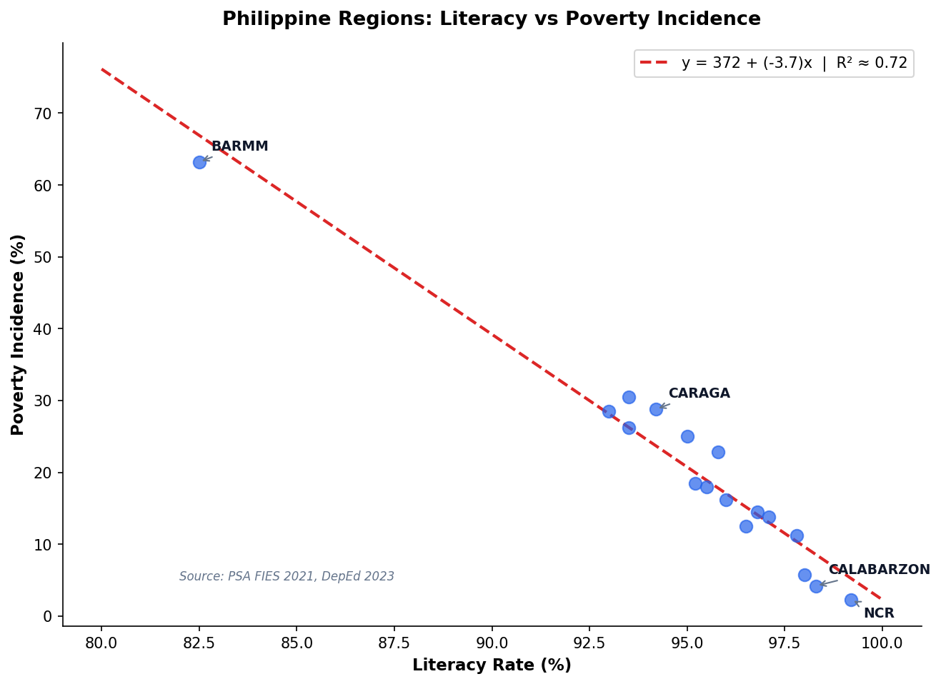
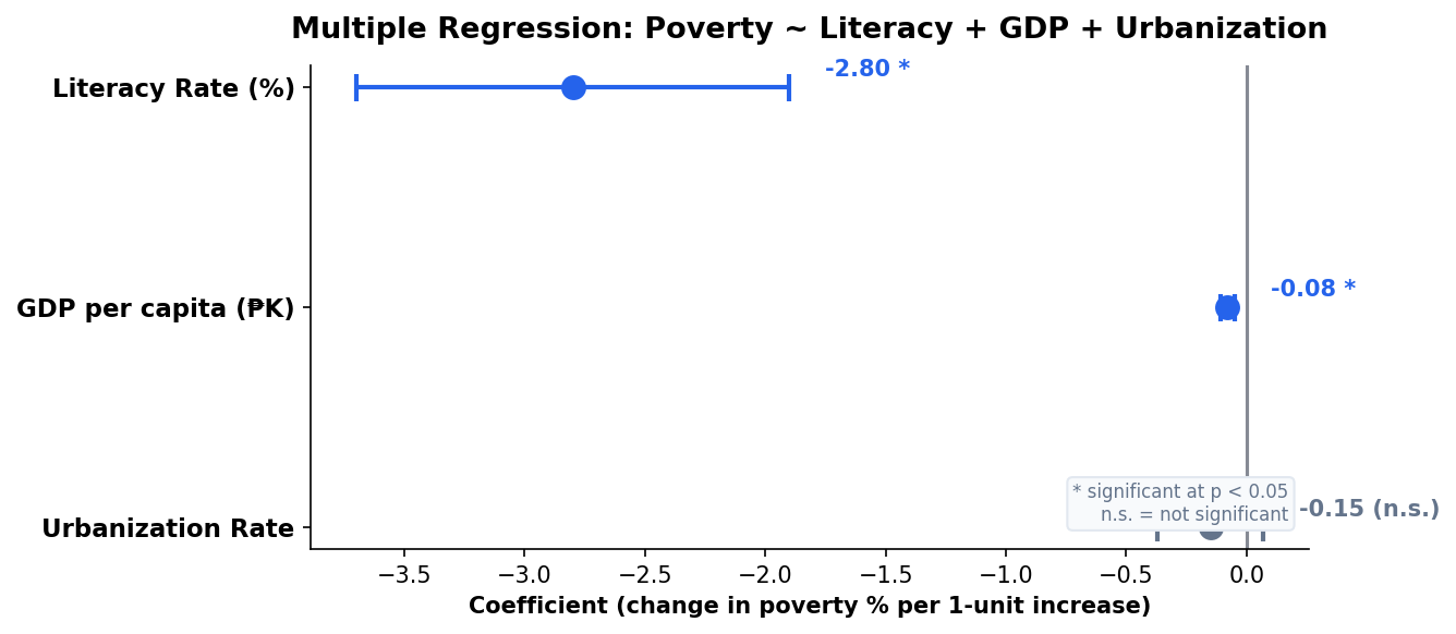
Multiple Predictors Paint a Richer Picture

Adding GDP per capita and urbanization rate to the literacy model:

PredictorCoeff.Note
Literacy Rate−2.80*Strongest predictor
GDP per capita−0.08*Significant but small effect
Urbanization−0.15Not significant after controlling for GDP

Key Insight

Urbanization becomes non-significant once GDP is in the model — suggesting urbanization’s effect on poverty operates through economic output, not independently.

Coefficient plot for multiple regression poverty model
Part III — Model Evaluation & Application

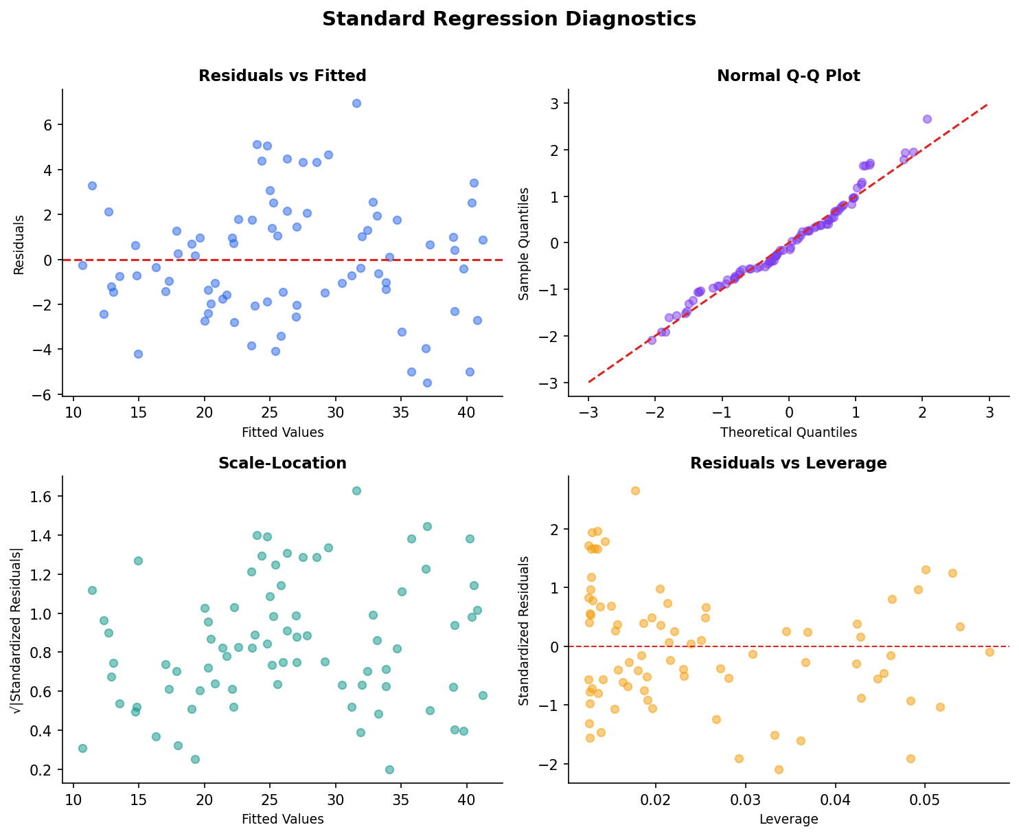
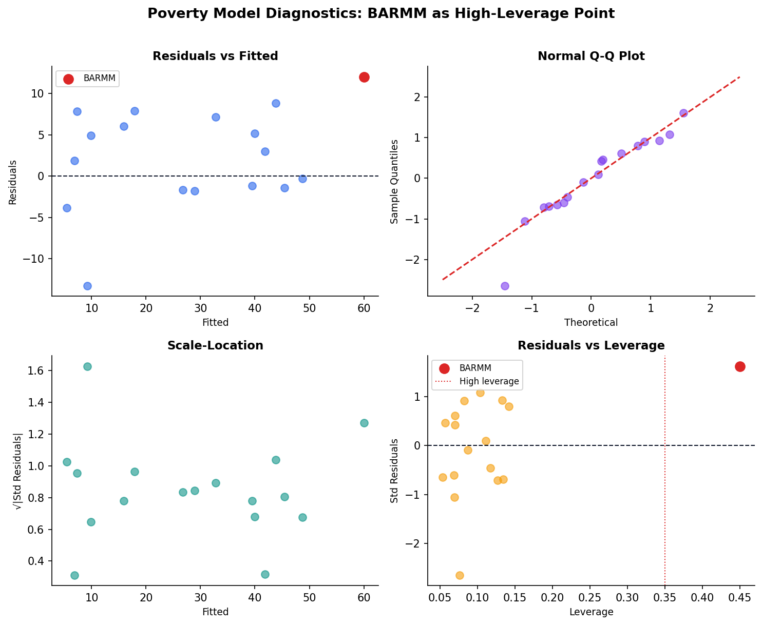
Diagnostics for the Poverty Model

Residual plot and leverage plot for Philippine poverty model
Part III — Model Evaluation & Application

Three Regression Pitfalls to Avoid

Overfitting

Too many predictors for your sample size. Rule of thumb: need 10–15 observations per predictor. With 17 Philippine regions, limit to 2–3 predictors.

"I added 8 predictors to a 17-row dataset and got R² = 0.99!"

Extrapolation

The model predicts well within the data range. Outside it, predictions are meaningless. Don’t predict poverty for a region with 70% literacy if your data only goes down to 82%.

"Our model says poverty would be −5% if literacy reached 100%."

Correlation ≠ Causation

Regression coefficients show association, not causation. Ice cream sales and drowning both rise in summer — regression would show a “significant” relationship.

"The data proves that ice cream causes drowning."

Part III — Model Evaluation & Application

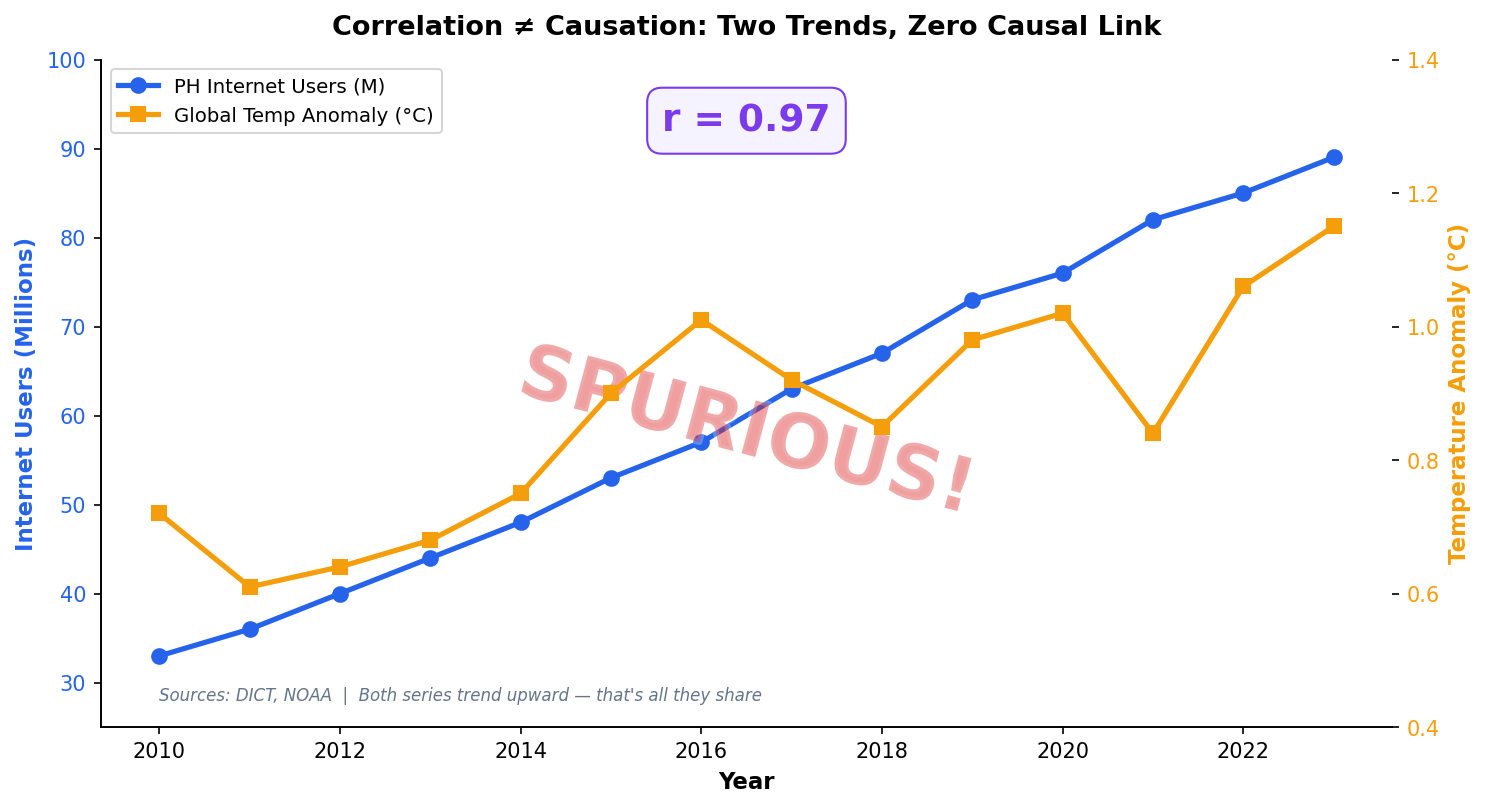
Correlation Does Not Imply Causation

A regression coefficient tells you that X and Y move together after controlling for other variables. It does not tell you that X causes Y.

When Can We Claim Causation?

Randomized controlled trials, natural experiments, or instrumental variables. Observational regression alone — no matter how high the R² — cannot prove causation.

The Analyst’s Responsibility

Always use language like “associated with” or “predicts,” never “causes” or “leads to,” when reporting regression results from observational data.

Spurious correlation example: ice cream vs drowning

Session 1 Key Takeaways

  1. Regression for analytics = interpretation first, prediction second.
  2. Every coefficient is a “holding all else constant” statement — translate it for stakeholders.
  3. Check LINE assumptions visually with residual plots before trusting any p-value.
  4. VIF > 10 means your coefficients are unreliable — drop or combine correlated predictors.
  5. The Philippine poverty model shows literacy, not urbanization, as the stronger lever.

Next: Session 2 — Logistic Regression & Classification

CMSC 178DA | Week 7 · Session 2

Logistic Regression:
Predicting Yes-or-No
Outcomes

From probabilities to decisions

Department of Computer Science

University of the Philippines Cebu

"Behind every automated approval is a probability and a threshold."

GCash approves or rejects 2 million loan applications per month.

Behind every decision is a logistic regression model trained on borrower features.

2M

decisions/month

0.5 sec

per decision

₱0

human review for standard cases

Agenda

Session 2 Objectives

Logistic Fundamentals

The sigmoid function, log-odds, and how to interpret odds ratios for stakeholders.

Classification Metrics

Confusion matrix, precision, recall, F1, and ROC-AUC — and when each matters most.

Decision-Making

Threshold tuning, cost-benefit analysis, and Philippine case studies in credit and education.

Part I

From Linear to Logistic

When the outcome is yes or no, linear regression breaks. The sigmoid function fixes it — and odds ratios make it interpretable.

Part I — From Linear to Logistic

Linear Regression Cannot Predict Probabilities

Linear regression vs logistic regression for binary outcome
Part I — From Linear to Logistic

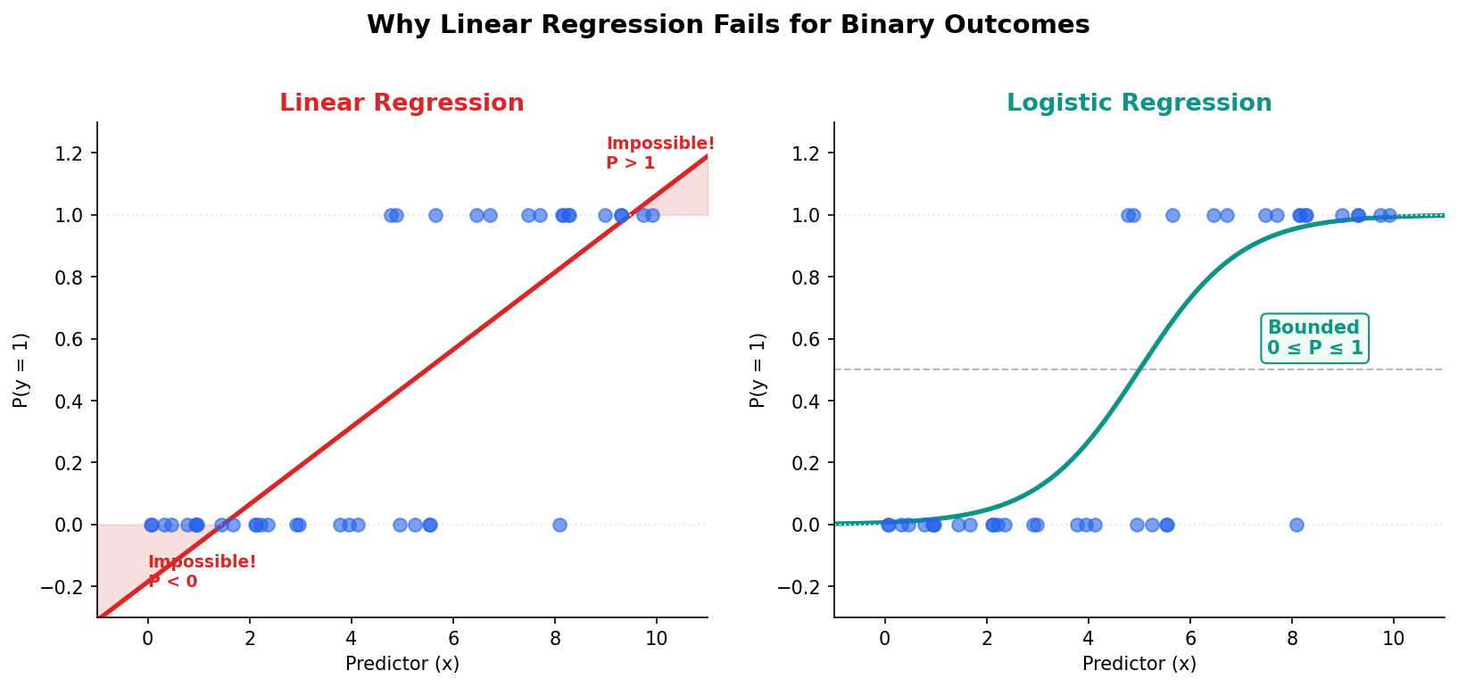
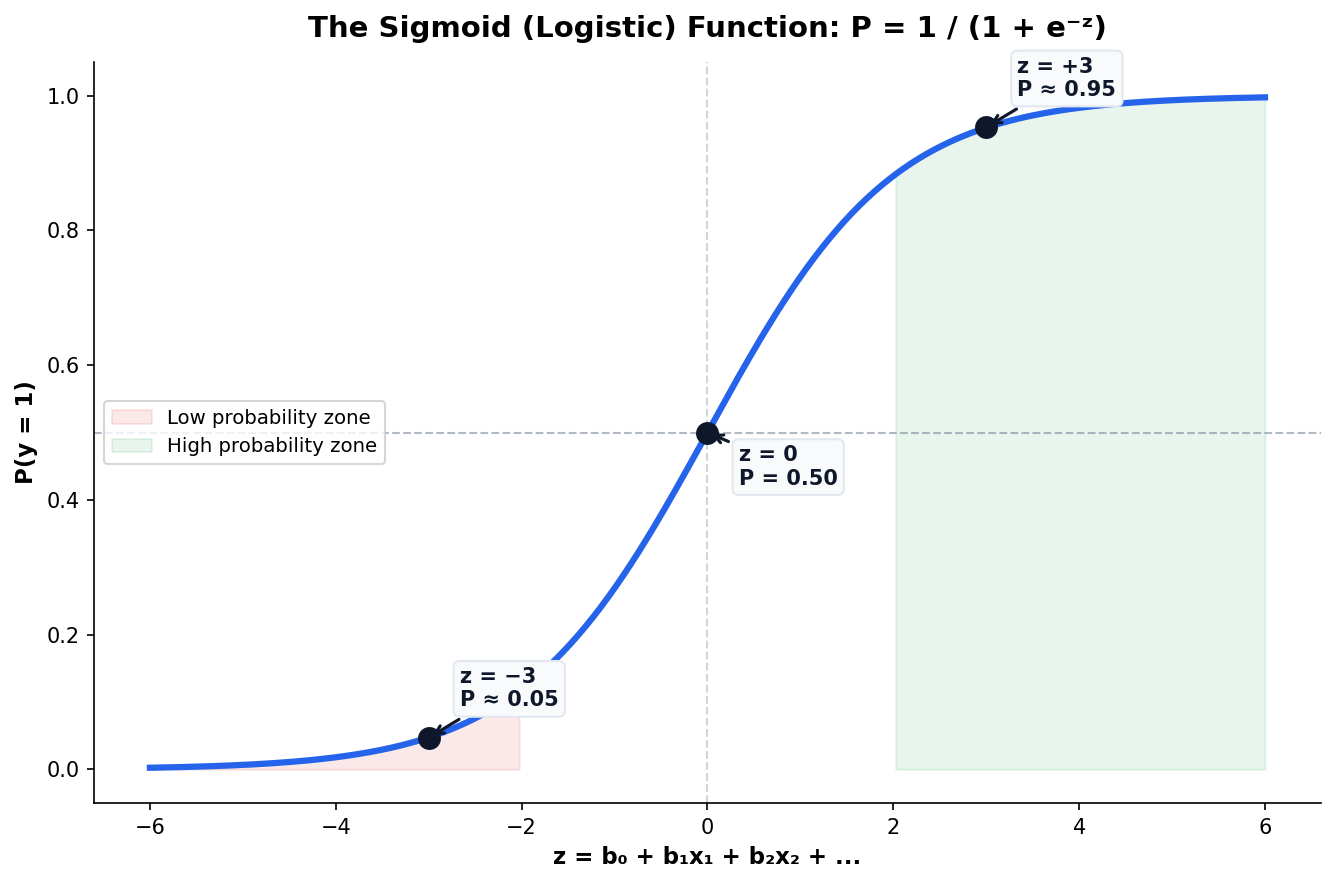
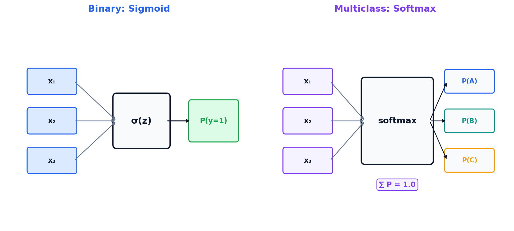
The Sigmoid Curve Maps Any Score to a Probability

The logistic function transforms any real-valued score z into a probability P between 0 and 1. The S-shape ensures smooth transitions near the decision boundary.

Why Sigmoid?

Natural for binary outcomes: as evidence increases, probability approaches 1 asymptotically but never exceeds it.

The Decision Boundary

Where P crosses 0.5 is the default classification threshold — but it’s rarely the optimal one for real problems.

Sigmoid S-curve with decision boundary at P=0.5
Part I — From Linear to Logistic

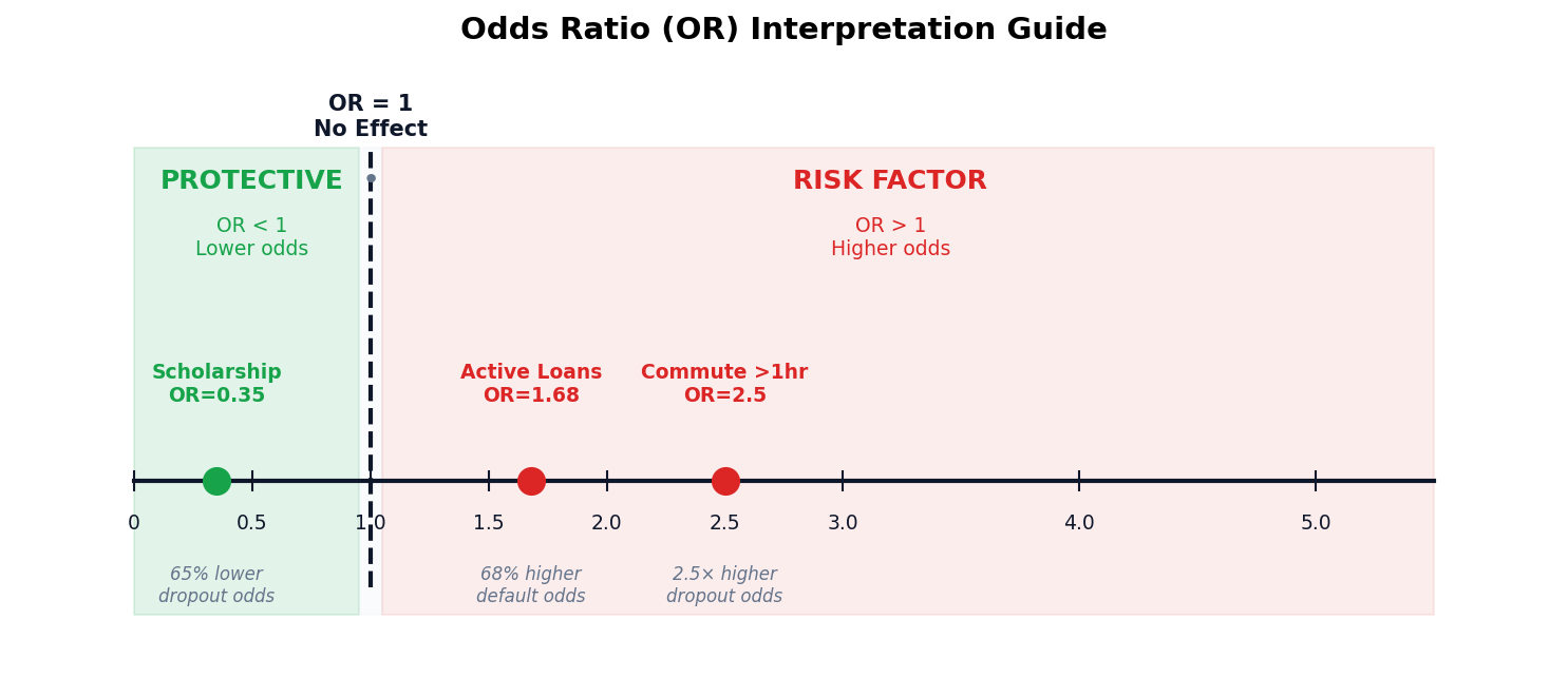
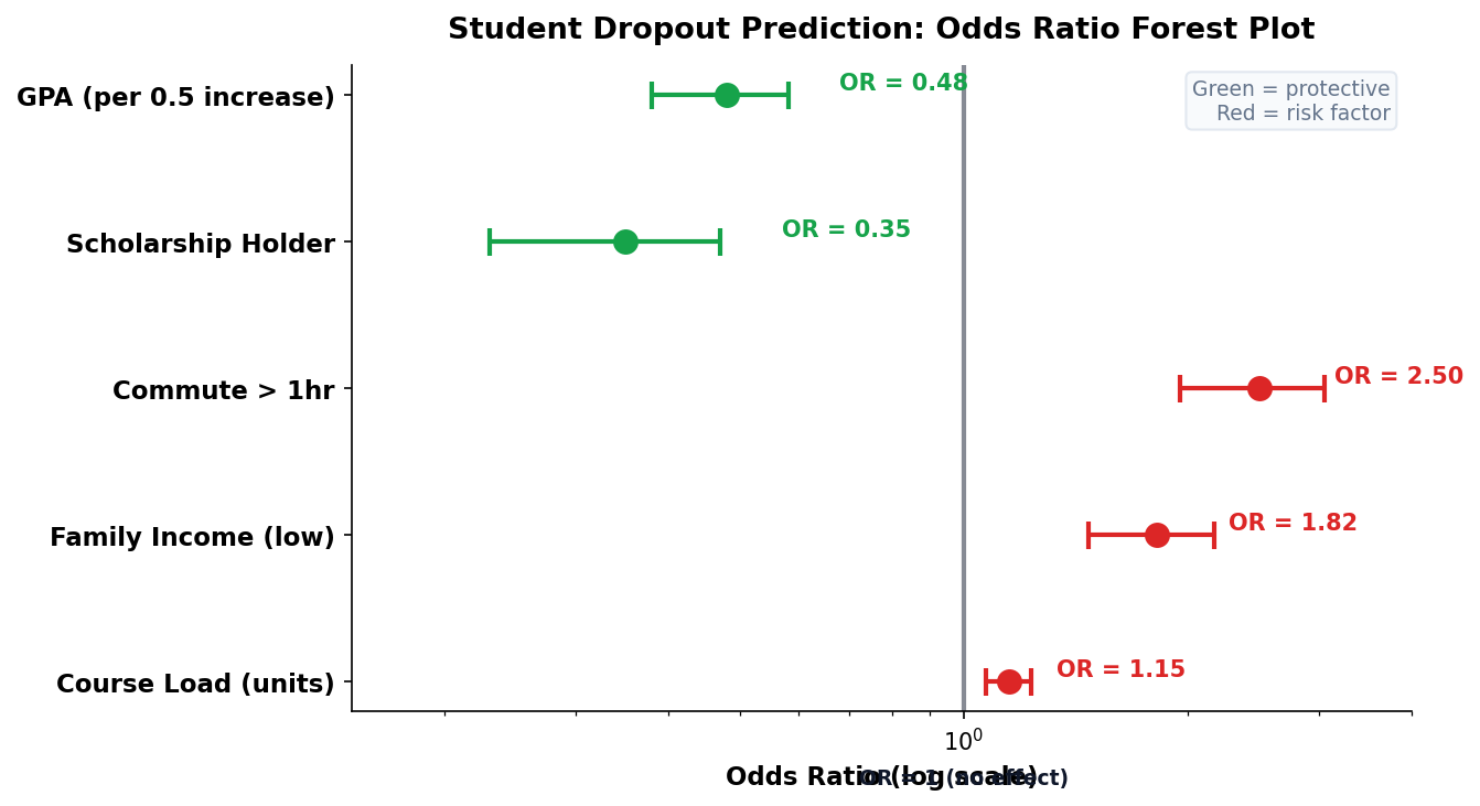
Odds Ratios Make Coefficients Interpretable

In logistic regression, we exponentiate the coefficient (e𝗛) to get the odds ratio. This tells stakeholders how much the odds change per unit increase in the predictor.

How to Read Odds Ratios

OR = 1: no effect. OR > 1: increases odds. OR < 1: decreases odds. OR = 2.5 means the odds are 2.5× higher for a 1-unit increase.

Example

A scholarship holder has OR = 0.35 for dropout — meaning 65% lower odds of dropping out compared to non-scholarship students.

Odds ratio forest plot with confidence intervals
Part I — From Linear to Logistic

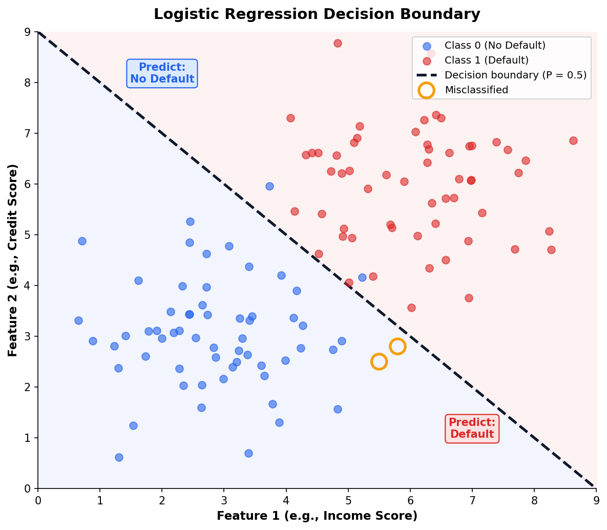
Decision Boundaries Separate the Outcomes

Decision boundary separating two classes in feature space
Part II

Measuring Classification Quality

Accuracy is a lie in imbalanced data. Precision, recall, and AUC tell the real story.

Part II — Measuring Classification Quality

The Confusion Matrix: Every Classifier’s Report Card

Confusion matrix with TP, FP, TN, FN labeled
Part II — Measuring Classification Quality

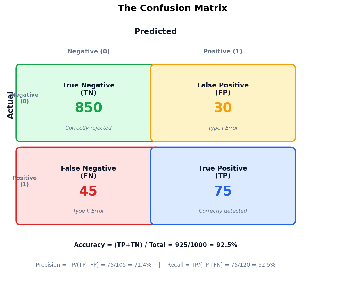
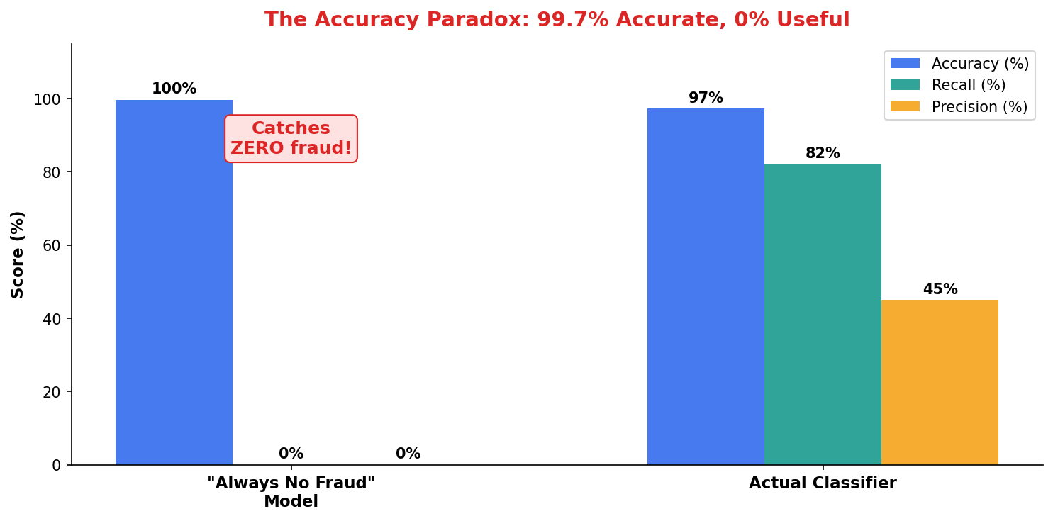
Accuracy Misleads When Classes Are Imbalanced

Accuracy paradox illustration with imbalanced dataset
Part II — Measuring Classification Quality

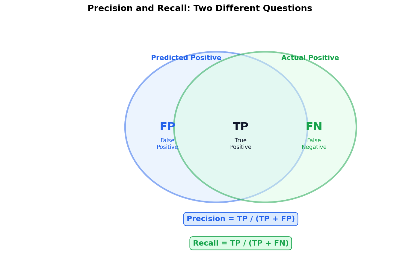
Precision and Recall Answer Different Questions

Precision asks: “Of everything I flagged, how much was correct?” Recall asks: “Of everything that was positive, how much did I catch?”

✓ High Precision Needed

Spam filter — don’t block legitimate email. Cost of FP > cost of FN.

× High Recall Needed

Disease screening — don’t miss sick patients. Cost of FN > cost of FP.

F1 Score

Harmonic mean of precision and recall. Use when you need to balance both and can’t afford to optimize one at the expense of the other.

Precision and recall Venn diagram
Part II — Measuring Classification Quality

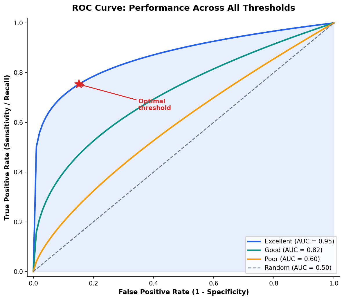
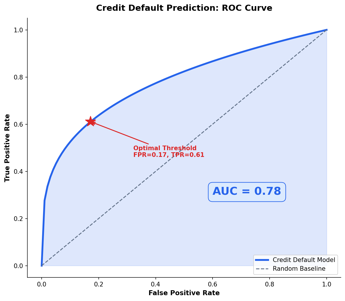
The ROC Curve Summarizes Performance Across All Thresholds

ROC curve with AUC shaded
Part II — Measuring Classification Quality

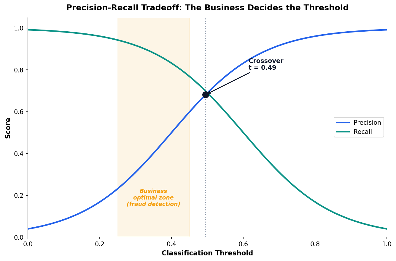
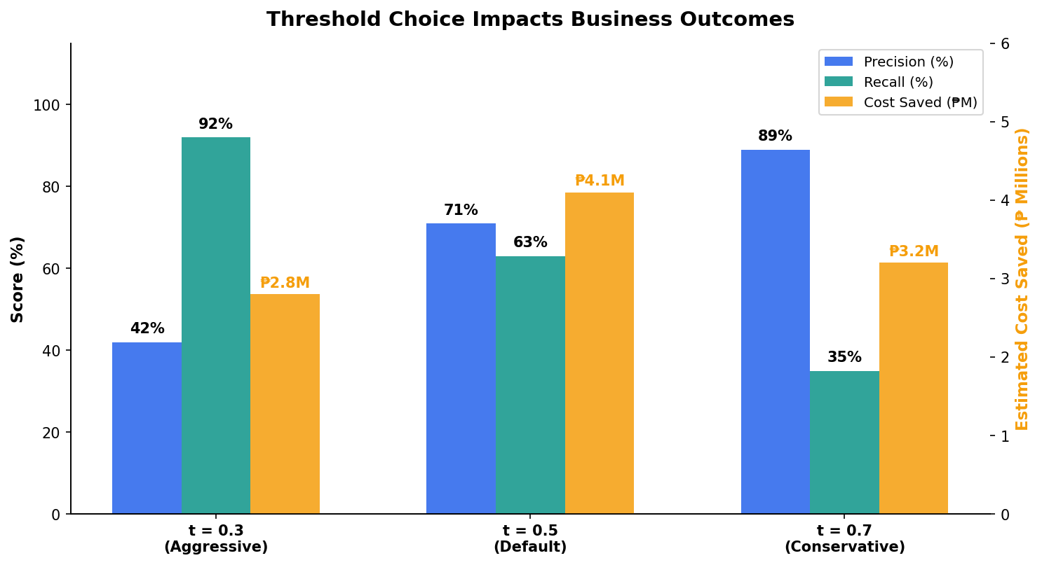
Threshold Tuning: The Business Decides, Not the Algorithm

Precision-recall tradeoff across different thresholds
Part III

Philippine Applications & What Comes Next

From credit scoring to student retention — logistic regression powers decisions across Philippine institutions.

Part III — Philippine Applications

Predicting Student Dropout: A UP Cebu Scenario

Student dropout logistic regression model results
Part III — Philippine Applications

Credit Default Prediction for Philippine Lenders

BSP-regulated consumer lending (GCash GLoan, Bayad Center) requires explainable models per BSP Circular 855.

FeatureORInterpretation
Monthly Income0.62Higher income → lower default odds
Outstanding Balance1.45Higher balance → higher risk
Employment Length0.78Longer tenure → lower risk
Active Loans1.68More loans → 68% higher default odds

Regulatory Context

BSP requires that lending models be explainable to regulators and consumers. Logistic regression’s odds ratios satisfy this requirement directly.

ROC curve for Philippine credit default model
Part III — Philippine Applications

From Odds Ratios to Actionable Recommendations

The analyst’s job: translate OR = 1.68 into “every additional active loan increases default risk by 68%.”

Decision Matrix

Low risk (P < 0.3): auto-approve. Medium (0.3–0.7): manual review. High (P > 0.7): auto-reject. Thresholds set by business, not by data science.

The Deliverable

A stakeholder-ready table mapping model output to business actions — not a confusion matrix.

Business impact chart showing cost at different thresholds
Part III — Philippine Applications

Multiclass Extension: Softmax Regression

When the outcome has more than two categories (e.g., customer segment A/B/C), the sigmoid extends to softmax — one probability per class, summing to 1.

Brief Mention

If you have 3+ classes, use softmax. For most analytics use cases, binary logistic regression covers the majority of decision problems.

Week 8 Preview

Decision trees handle multiclass naturally and don’t require the linearity assumption. Next week we explore when trees beat regression.

Softmax function mapping inputs to multiclass probabilities
Part III — Philippine Applications

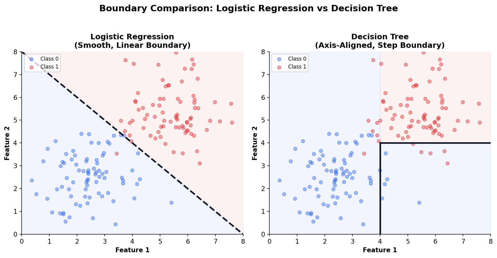
Logistic Regression vs Decision Trees: When to Use Which

Both can classify. The choice depends on your data and your audience.

CriterionLogistic RegressionDecision Tree
InterpretabilityCoefficients + ORIf-then rules
Feature TypesNumeric (needs encoding)Numeric + categorical natively
LinearityAssumes linear log-oddsNo linearity assumption
InteractionsMust add manuallyDiscovers automatically
SpeedVery fastFast (slower for ensembles)

Preview

Next week we explore decision trees, random forests, and gradient boosting — and when they outperform logistic regression.

Side-by-side logistic regression vs decision tree boundaries
Part III — Philippine Applications

Three Logistic Regression Mistakes to Avoid

Using Accuracy on Imbalanced Data

Always check class balance first. If 99% of cases are negative, accuracy is useless. Use F1, AUC, or precision-recall instead.

"Our fraud model has 99.7% accuracy!" — it predicts “no fraud” for everything.

Ignoring Odds Ratio Direction

OR = 0.5 means protective (50% lower odds), not harmful. Misreading direction leads to exactly wrong recommendations.

"OR = 0.35, so scholarships increase dropout risk!" — it’s the opposite.

One Threshold for All

Different business contexts require different thresholds. Fraud detection (low threshold) ≠ churn prediction (balanced) ≠ medical screening (very low).

"We use 0.5 for everything." — one size never fits all.

Session 2 Key Takeaways

  1. Logistic regression predicts probabilities for binary (yes/no) outcomes — bounded between 0 and 1.
  2. Odds ratios (e𝗛) make coefficients interpretable for stakeholders — no math degree required.
  3. Accuracy lies in imbalanced data — always check precision, recall, F1, and AUC.
  4. Threshold choice is a business decision, not a statistical one — align it with the cost of errors.
  5. Decision trees (Week 8) handle non-linear boundaries and multiclass outcomes naturally.

Next Week: Tree-Based Methods — Decision Trees, Random Forests, and Gradient Boosting

Week 8 Preview

Tree-Based Methods

Decision Trees — interpretable if-then rules

Random Forests — ensemble power

Gradient Boosting — state-of-the-art tabular performance

Lab 7: Build a Philippine credit scoring model, interpret odds ratios, and optimize the threshold for a business objective.