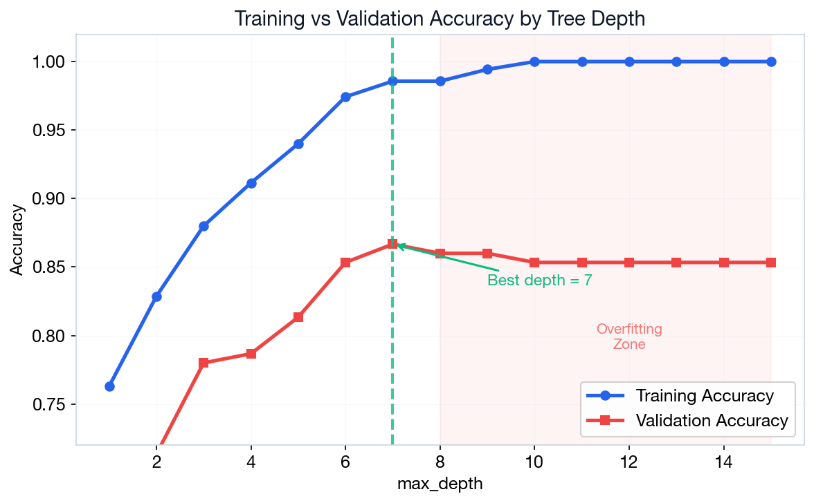
The Most Interpretable Machine Learning Model
Department of Computer Science
University of the Philippines Cebu
Lecture 15: CART, Pruning & Interpretation
Learn the CART algorithm and how it splits data using Gini impurity and entropy.
Read tree visualizations and extract business rules from trained models.
Use pre-pruning and post-pruning to prevent overfitting.
Recognize when decision trees outperform other methods.
Three properties that make decision trees uniquely valuable in data analytics.
Visual structure mirrors human decision-making. Non-technical stakeholders can understand the model.
Handles non-linear relationships without feature transformations or polynomial terms.
No feature scaling required. Automatic feature selection. Handles mixed data types natively.
A decision tree is a flowchart of binary decisions, splitting data at each node until reaching a prediction.
A greedy, recursive algorithm that finds the best binary split at each node.
Greedy = picks the best split right now without looking ahead. Fast, but not guaranteed globally optimal.
Binary Split = every node asks one yes/no question (e.g., "Age ≤ 35?"). Data always splits into exactly two groups.
Given 6 loan applicants, CART evaluates every possible split and picks the one with the lowest weighted Gini.
| Age | Income | Savings? | Approved? |
|---|---|---|---|
| 25 | ₱30K | Yes | Yes |
| 45 | ₱80K | No | No |
| 35 | ₱50K | Yes | Yes |
| 22 | ₱20K | No | No |
| 50 | ₱90K | Yes | Yes |
| 28 | ₱35K | No | No |
Try 1: "Age ≤ 30?" → Left: [Y, N, Y], Right: [N, Y, N] → Weighted Gini = 0.444
L(3): 1−(0.667²+0.333²)=0.444 R(3): same Weighted: (3/6)×0.444+(3/6)×0.444=0.444
Try 2: "Income ≤ ₱50K?" → Left: [Y, N, Y, N], Right: [N, Y] → Weighted Gini = 0.333
Try 3: "Has Savings?" → Left: [Y, Y, Y], Right: [N, N, N] → Weighted Gini = 0.000 ✓
CART picks "Has Savings?" because it produces the lowest weighted Gini. Pure leaves = perfect separation. This is what greedy means — pick the best split NOW.
Gini = 1 − Σ pi²
Why p²? pi² = chance two random picks are both class i. So 1−Σpi² = chance they disagree = impurity.
Example: 8 samples: 6 cats, 2 dogs. pcat=0.75, pdog=0.25.
Gini = 1 − (0.75² + 0.25²) = 1 − 0.625 = 0.375
Entropy = −Σ pi log2(pi)
Example: Same node. Entropy = −(0.75 × log20.75 + 0.25 × log20.25)
= −(−0.311 + −0.500) = 0.811
1. Parent node: 10 samples (6 Yes, 4 No)
Gini = 1 − (0.6² + 0.4²) = 1 − 0.52 = 0.48
2. Split "Age ≤ 30":
Left child (4 samples): 3 Yes, 1 No → Gini = 1 − (0.75² + 0.25²) = 0.375
Right child (6 samples): 3 Yes, 3 No → Gini = 1 − (0.5² + 0.5²) = 0.500
3. Weighted Gini:
(4/10) × 0.375 + (6/10) × 0.500 = 0.15 + 0.30 = 0.45
4. Information Gain = Parent impurity − Weighted child impurity — how much a split reduces disorder.
0.48 − 0.45 = 0.03 (small improvement — CART tries other splits to find a better one)
from sklearn.tree import DecisionTreeClassifier, plot_tree
clf = DecisionTreeClassifier(
max_depth=3,
random_state=42
)
# X_train = feature matrix (rows=samples, cols=features)
# y_train = labels (the class we are predicting)
clf.fit(X_train, y_train)
# Visualize the trained tree
plot_tree(clf,
feature_names=features,
class_names=['Reject', 'Approve'],
filled=True, rounded=True)
Output → The tree diagram on the right. Each node shows the split condition, Gini, sample count, and class distribution.
Each node in a sklearn tree visualization shows five key pieces of information.
Feature & thresholdAge <= 35.5
Impurity measuregini = 0.42
Training examplessamples = 150
Class distributionvalue = [30, 70]
Majority predictionclass = Yes
Unconstrained decision trees memorize training data, creating overly complex structures that fail to generalize.
Constrain the tree during training with hyperparameters.
Absolute depth limit. Start: 5–10
Min samples to attempt split. Start: 10–20
Min samples for a valid leaf. Start: 5–10
Max features per split. Start: ‘sqrt’
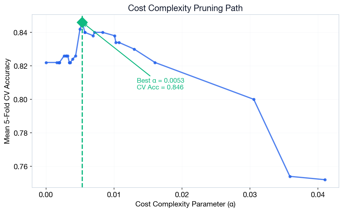
Grow a full tree, then prune branches that don't improve generalization.
Rα(T) = R(T) + α|T|
Example: R(T)=0.15, |T|=8, α=0.01 → Cost = 0.15 + 0.01×8 = 0.23.
Prune to 4 leaves: R(T)=0.18, Cost = 0.18 + 0.01×4 = 0.22 (lower → prune!)
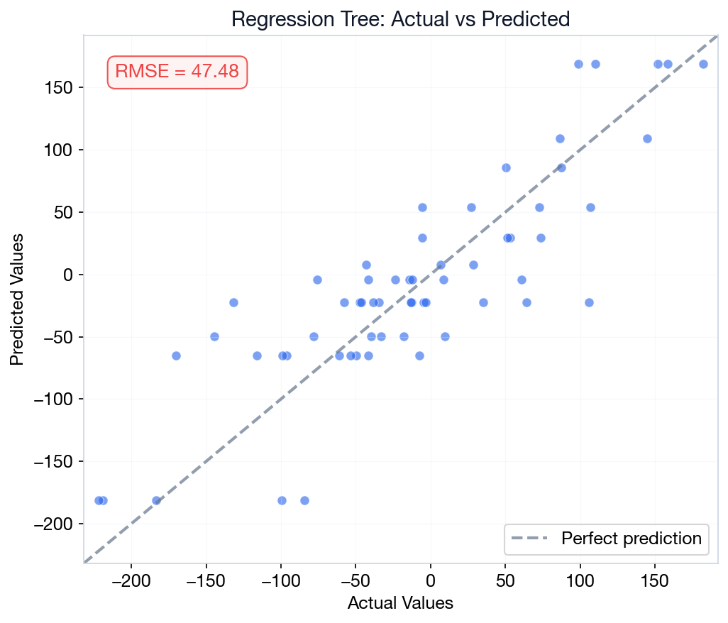
Importance = total reduction in impurity contributed by each feature across all splits.
Each split reduces impurity. Features used in higher, more impactful splits accumulate greater importance scores.
Trees aren't always the answer, but in these three scenarios they often outperform.
Excel-style data with mixed types (categorical + continuous). Neural networks struggle here.
Finance, healthcare, insurance — interpretability is legally required.
Trees excel with limited data. Neural networks need massive datasets to generalize.
Same tree structure, but leaf values are means instead of class labels. Splits minimize MSE within each partition.
Classification: leaf = majority class vote.
Regression: leaf = mean of training samples in
that partition.
Example: A leaf contains 5 houses priced at: ₱2M, 2.5M, 3M, 2.8M, 2.2M
Prediction = mean = (2 + 2.5 + 3 + 2.8 + 2.2) / 5 = ₱2.5M
MSE: CART finds the cut that minimizes price variance in each child group. Lower variance = more similar houses grouped together.
Build an interpretable loan approval model using Philippine bank data. Extract human-readable rules for credit officers.
Decision trees let loan officers explain why an application was approved or rejected — critical for BSP compliance.
Convert the trained tree into actionable IF-THEN rules for stakeholders.
|--- credit_score <= 650 | |--- income <= 250k | | |--- class: Reject | |--- income > 250k | | |--- emp_years <= 2 | | | |--- class: Review | | |--- emp_years > 2 | | | |--- class: Approve |--- credit_score > 650 | |--- class: Approve
Credit score > 650 = Fast-track auto-approve. No need to check other features.
Small changes in training data produce very different trees.
Only perpendicular cuts. Struggles with diagonal decision boundaries.
Makes locally optimal splits, may miss globally optimal structure.
Combine many trees into Ensemble Methods (next lecture).
A Decision Tree predicting loan defaults achieves 99.8% Training Accuracy but only 62% Validation Accuracy. What is the most likely cause?
Click to reveal answer
Correct: C (Overfitting)
A massive gap between training and validation accuracy is the textbook definition of overfitting. The tree has grown too deep and memorized specific training examples. Solution: Prune it!
1. Decision trees are the most interpretable ML model — stakeholders can read the rules directly.
2. CART uses Gini impurity or entropy to find the best binary split at each node.
3. Pruning (pre & post) prevents overfitting by constraining tree complexity.
4. Single trees have high variance — next lecture: ensemble methods fix this.
Combine many decision trees to overcome the limitations of a single tree.
pip install xgboost lightgbm shapCombining Trees for Superior Performance
Department of Computer Science
University of the Philippines Cebu
Lecture 16: Ensembles, XGBoost & SHAP
Understand bagging, boosting, and stacking paradigms.
Apply Random Forest for robust, low-variance predictions.
Use XGBoost and LightGBM for state-of-the-art tabular ML.
Explain individual model predictions with SHAP values.
Ensemble (French for “together”) = train multiple models and combine their predictions. Like asking 100 doctors instead of 1 — the group answer is usually better than any individual.
Train on random data subsets (with replacement), then average predictions. Reduces variance.
Train models sequentially — each one fixes mistakes of the previous. Reduces bias.
Train different model types, then a “meta-model” learns the best way to combine them.
E[Error] = Bias2 + Variance + σ2irreducible
Bias = error from oversimplifying. A straight line fitting curved data.
Variance = error from being too sensitive. Tiny data changes → wildly different predictions.
σ² = noise in the data itself. No model can remove it.
| Method | Bias | Variance | Strategy |
|---|---|---|---|
| Single Tree | Low | High | Memorizes (Overfits) |
| Bagging | Low | Reduced | Averages many trees |
| Boosting | Reduced | Low | Corrects errors |
Build many trees on different bootstrap samples, with random feature subsets at each split.
m = √p (classification) | m = p/3 (regression)
m = features per split, p = total features
Bootstrap sample: Draw n rows with replacement from n rows. Some rows repeat; ~37% are never selected — those become the OOB validation set.
Correlated trees don't help. If one feature dominates (e.g., income), all trees will use it at the root — producing near-identical trees.
Force each split to choose from a random subset of features. This creates diverse, uncorrelated trees whose errors cancel out.
'sqrt' — for classification'log2' or 1/3 — for regressionMore diversity = better ensemble. Random subsets force each tree to learn different patterns.
from sklearn.ensemble import RandomForestClassifier
rf = RandomForestClassifier(
n_estimators=200, # 200 trees
max_features='sqrt', # sqrt(p) features/split
oob_score=True, # free validation
n_jobs=-1, # all CPU cores
random_state=42
)
rf.fit(X_train, y_train)
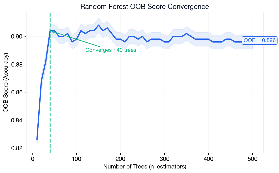
print(f"OOB Score: {rf.oob_score_:.3f}")
Output: OOB converges around 0.92 (see right). Diminishing returns after ~200 trees.
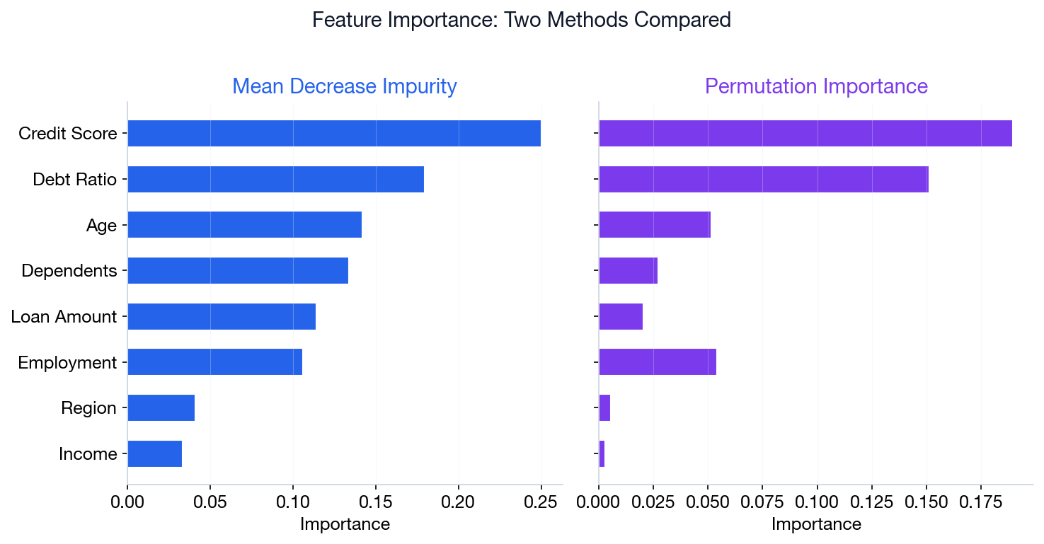
Built-in, fast, but biased toward high-cardinality features (high-cardinality = many unique values, e.g. ZIP codes).
rf.feature_importances_ — sum of Gini decreases across all trees where the feature is used.
More reliable. Measures accuracy drop when feature values are shuffled.
permutation_importance(rf, X_test, y_test) — model-agnostic, works with any estimator.
MDI for quick screening during development. Permutation for final reports — it’s unbiased and works on any model, not just trees.
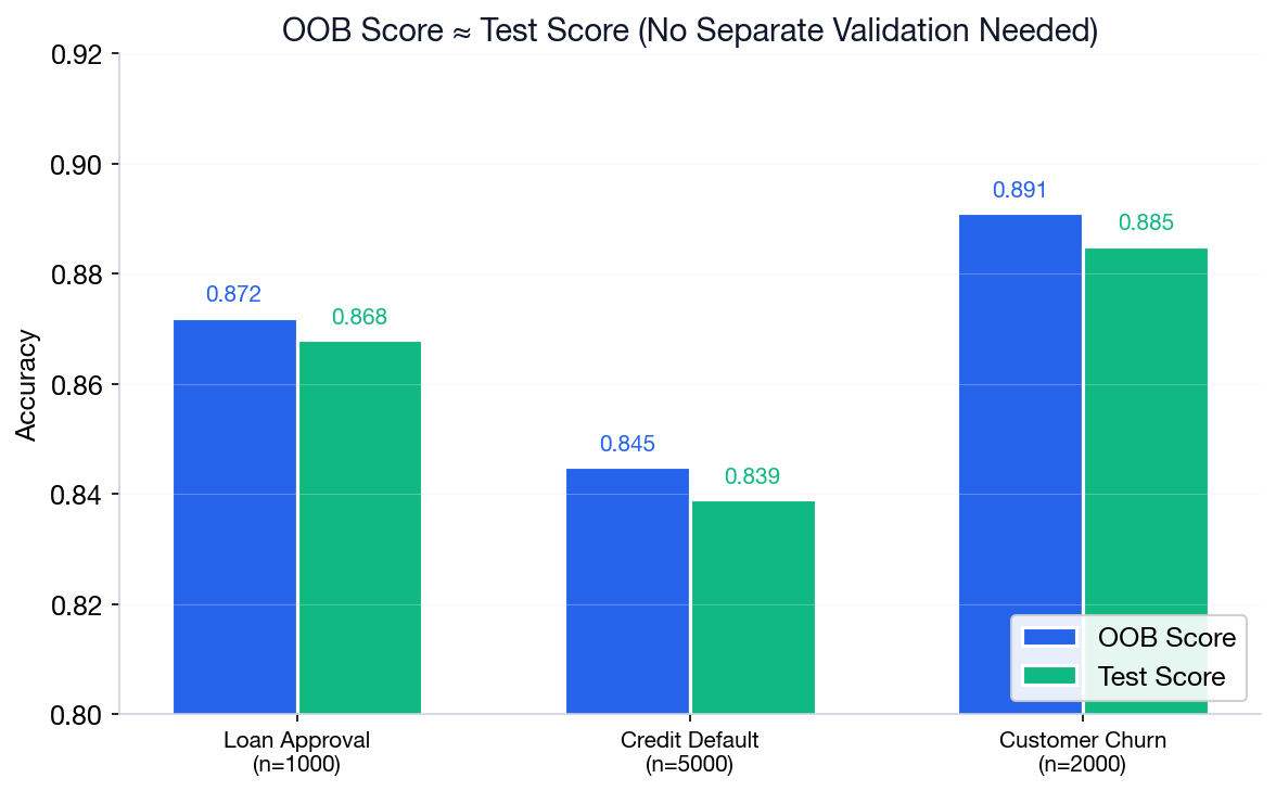
Each tree is trained on ~63% of data (bootstrap sample). The remaining ~37% can be used as a free validation set.
P(not selected) = (1 − 1/n)n ⟶ 1/e ≈ 0.368
~63.2% in-bag • ~36.8% out-of-bag (free validation)
No need for a separate validation set! OOB score approximates test performance without holding out data.
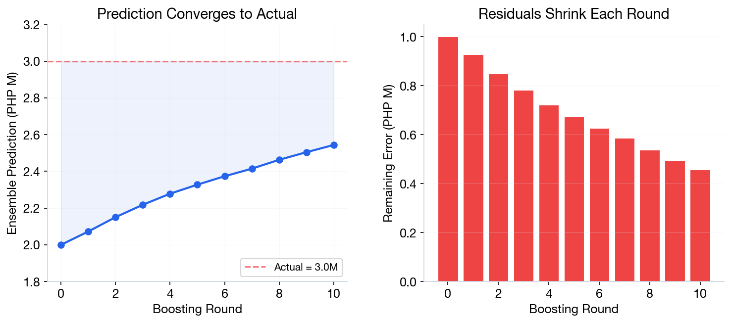
Each new tree focuses on the mistakes of the previous ensemble.
Weak learner = a model barely better than random guessing (typically a depth-1 tree, called a “stump”).
Residual = actual − predicted. If actual = 100 and predicted = 85, residual = 15.
Bagging = parallel, reduces variance. Boosting = sequential, reduces bias.
Predicting a house price. Actual = ₱3.0M
| Iter | What Tree Learns | Output | Running Total |
|---|---|---|---|
| 0 | Start: mean of all prices | — | ₱2.0M |
| 1 | Residual: 3.0 − 2.0 = 1.0M | +0.8M | ₱2.8M |
| 2 | Residual: 3.0 − 2.8 = 0.2M | +0.15M | ₱2.95M |
| 3 | Residual: 3.0 − 2.95 = 0.05M | +0.04M | ₱2.99M |
Each tree corrects the remaining error. After just 3 iterations: ₱2.0M → ₱2.99M — almost perfect!
Notice: Output < Residual each round. That gap is the learning rate (γ) — it scales how much each tree contributes. (Defined formally on the next slide.)
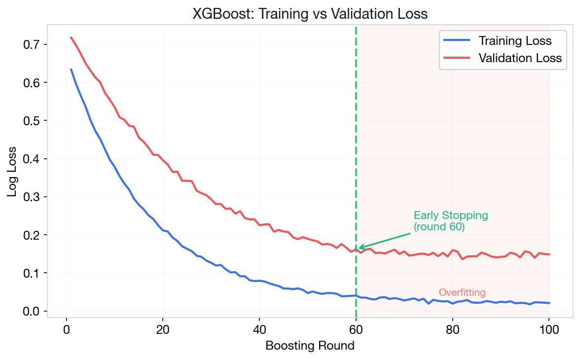
Each new tree only predicts the leftover errors. Final prediction = sum of all trees' contributions.
Fm(x) = Fm−1(x) + γm hm(x)
Example: Old prediction = 85, new tree says error = +12, γ = 0.1 → new prediction = 85 + 0.1 × 12 = 86.2
Fast, regularized, scalable. The go-to algorithm for Kaggle competitions and production ML on tabular data.
Built-in L1/L2 regularization, early stopping, missing value handling, and parallel tree construction.
| n_estimators | Number of boosting rounds (100–1000) |
| learning_rate | Step size shrinkage (0.01–0.3) |
| max_depth | Tree depth (3–10, default 6) |
| early_stopping | Stop when validation loss plateaus |
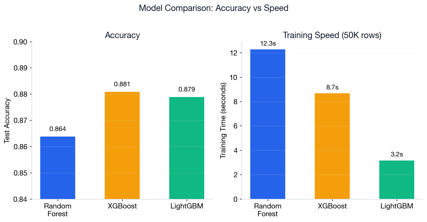
Choose XGBoost when: you need maximum accuracy on tabular data and can invest time in hyperparameter tuning. Use Random Forest when you need a robust model with minimal tuning.
import xgboost as xgb
model = xgb.XGBClassifier(
n_estimators=200,
max_depth=6,
learning_rate=0.1,
early_stopping_rounds=10,
eval_metric='logloss' # penalizes overconfident wrong predictions
)
model.fit(X_train, y_train,
eval_set=[(X_val, y_val)],
verbose=False)
print(f"Best round: {model.best_iteration}")
print(f"Test acc: {model.score(X_test, y_test):.3f}")
Early Stopping = stop training when validation loss stops improving. Prevents overfitting automatically.
logloss = penalizes overconfident wrong predictions (lower = better).
L1 reg = drives small weights to zero (implicit feature selection). L2 reg = shrinks all weights evenly, prevents any one feature dominating.
import lightgbm as lgb
model = lgb.LGBMClassifier(
n_estimators=200,
num_leaves=31, # main complexity control
learning_rate=0.1,
n_jobs=-1
)
model.fit(X_train, y_train)
Leaf-wise vs Level-wise: XGBoost grows all nodes at the same depth (level-wise). LightGBM grows the leaf that reduces loss the most (leaf-wise) — faster, but can overfit on small data.
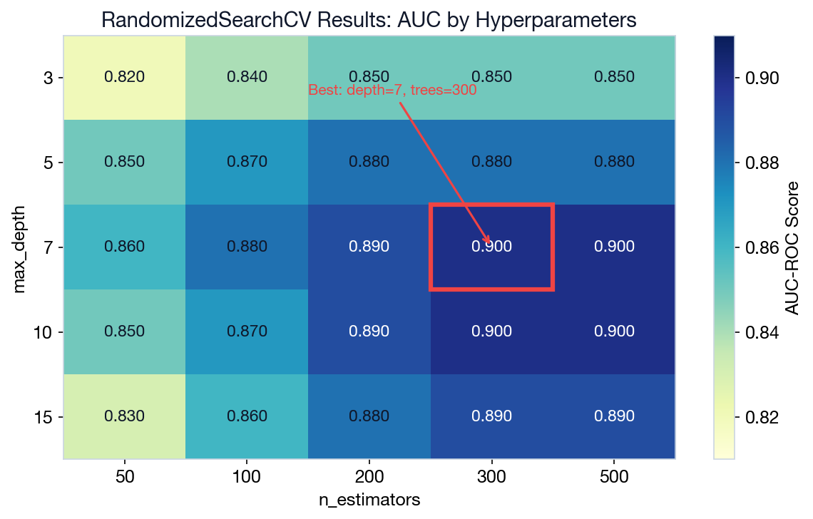
| Aspect | Random Forest | Gradient Boosting |
|---|---|---|
| Training | Parallel (fast) | Sequential (slower) |
| Overfitting | Less prone | More prone |
| Tuning | Easier (fewer params) | More hyperparameters |
| Performance | Good baseline | Often best |
| Best For | Quick baseline, noisy data | Maximum accuracy, competitions |
Start with Random Forest as a baseline. Switch to XGBoost/LightGBM when you need extra performance.
from sklearn.model_selection import RandomizedSearchCV
param_dist = {
'n_estimators': [100, 200, 300, 500],
'max_depth': [3, 5, 7, 10],
'learning_rate': [0.01, 0.05, 0.1],
}
search = RandomizedSearchCV(
xgb.XGBClassifier(), param_dist,
n_iter=20, cv=5, scoring='roc_auc'
)
search.fit(X_train, y_train)
print(search.best_params_)
Use scoring='roc_auc' for imbalanced datasets. RandomizedSearchCV is much faster than GridSearch when the parameter space is large.
cv=5 = 5-fold cross-validation: split data into 5 parts, train on 4, test on 1, repeat 5×, average the scores.
roc_auc = Area Under ROC Curve. Measures class separation ability. 1.0 = perfect, 0.5 = random guessing.
Intuition: Imagine a team project. SHAP figures out each member's (feature's) fair contribution to the final grade (prediction). It asks: “If we remove this feature, how much does the prediction change?”
φi = ∑S⊆N\{i} |S|!(|N|−|S|−1)! ⁄ |N|! · [v(S∪{i}) − v(S)]
Marginal contribution of feature i, averaged over all coalitions (coalition = any subset of features used together)
Feature importance tells you which features matter globally. SHAP tells you why a specific prediction was made.
How to read beeswarm: Red dots right = pushes prediction up. Blue dots left = pushes down. Wider spread = more important.
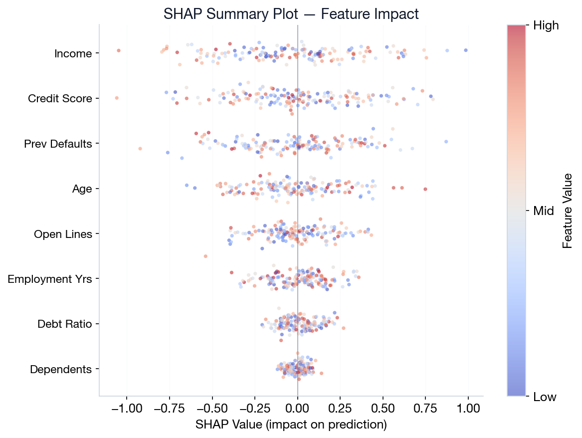
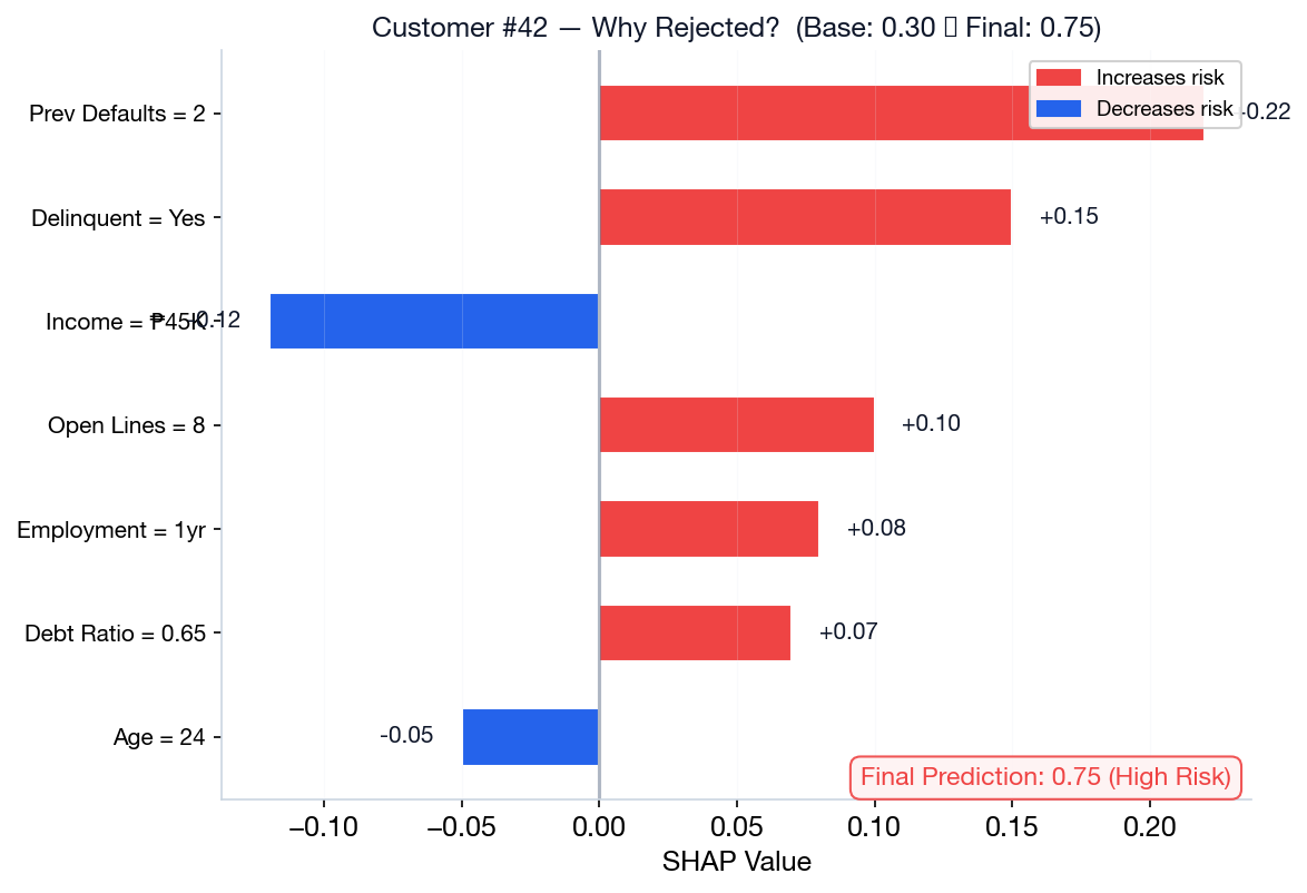
Base prediction (average across all applicants) = 30% risk. Each feature nudges the prediction up or down.
| Feature | Value | SHAP Impact | Running Total |
|---|---|---|---|
| Base prediction | — | — | 0.30 |
| + Previous Defaults | 2 | +0.22 | 0.52 |
| + Delinquent | Yes | +0.15 | 0.67 |
| + Open Credit Lines | 8 | +0.10 | 0.77 |
| − Income | ₱120K | −0.12 | 0.65 |
| + Debt Ratio | 0.65 | +0.07 | 0.72 |
| Final Prediction | — | — | 0.72 (High Risk) |
The final prediction (72% risk) = base + all SHAP values summed. Each feature has a signed contribution: positive pushes risk up, negative pushes it down.
This is exactly what the waterfall plot on the next slide visualizes.
Each bar shows how one feature shifts the prediction from the base value.
Build a credit scoring model on Philippine data and explain individual rejection decisions using SHAP.
Simulated Philippine credit data: income, employment length, number of open credit lines, previous defaults, delinquency status. Target: default risk (binary).
SHAP explanations satisfy BSP regulatory requirements for transparent credit decisions.
When building a model on a tabular dataset, in which scenario would you strongly prefer XGBoost over Random Forest?
Click to reveal answer
Correct: A (Maximizing Accuracy)
Boosting models (XGBoost) actively correct residuals sequentially, often leading to higher performance on tabular data. Random Forest is preferred when you need lower tuning effort and high stability against outliers.
1. Ensembles combine multiple models to reduce variance (bagging) or bias (boosting).
2. Random Forest uses bagging + feature randomization for robust, easy-to-tune models.
3. XGBoost & LightGBM are state-of-the-art for tabular data, with built-in regularization.
4. SHAP values explain individual predictions — critical for regulated industries.
Build the best predictive model for a Philippine dataset using tree-based methods.
| Algorithm | Tuning Effort | Speed | Accuracy | Your Goal |
|---|---|---|---|---|
| Decision Tree | Low | Fast | Baseline | Set the floor |
| Random Forest | Low–Medium | Fast (parallel) | Good | Beat the baseline |
| XGBoost | Medium–High | Medium | Best | Win the competition |
| LightGBM | Medium | Fastest | Best | Alternative to XGB |
Next Week: Clustering & Segmentation — K-Means, Hierarchical Clustering, DBSCAN, and Customer Analytics.