CMSC 178DA | Week 10 — Session 1

Predicting the Future with Data

Time Series Fundamentals

Department of Computer Science

University of the Philippines Cebu

Lecture 19: Fundamentals & Smoothing

Every Quarter, $8.9 Billion Flows into the Philippines

OFW remittances follow the same seasonal pattern year after year.

~8% of Philippine GDP

2.2M OFWs abroad

Dec peak every year

This repeating pattern is a time series. Today we learn to analyze it.

Agenda

Session 1 Objectives

Components

Decompose time series into trend, seasonality, and residuals.

Stationarity

Test and transform data for forecasting readiness using ADF and differencing.

Smoothing

Apply moving average and exponential smoothing methods to extract signal from noise.

Running Example

Meet Our Data: OFW Remittances

We'll use monthly Philippine OFW remittance data throughout both sessions. Real BSP data — small enough to trace by hand, big enough to show real patterns.

Three Patterns to Spot

Trend (long-term direction of the data) — remittances grow ~4% per year
Seasonality (repeating pattern at fixed intervals) — December peak (Christmas!)
Noise (random, unpredictable variation) — random monthly fluctuation

Challenge

Look at the table. Can you guess what January 2024 will be? That's exactly what our algorithms will learn to do.

Month	Remittances (B USD)	Pattern
Jan 2023	7.8
Feb 2023	7.5
Mar 2023	8.0
Apr 2023	7.9
May 2023	8.2
Jun 2023	8.1
Jul 2023	8.4
Aug 2023	8.3
Sep 2023	8.5
Oct 2023	8.7	↗ trend
Nov 2023	8.9	↗ trend
Dec 2023	9.8	↑ seasonal peak!

Source: BSP (Bangko Sentral ng Pilipinas). Values illustrative.

Part I

What Makes Time Unique

Unlike cross-sectional data, time series carries memory. Today depends on yesterday.

This section covers time series structure, decomposition, and resampling.

Video Resource

Common Time Series Patterns

Watch this 5-minute overview before we dive into each pattern. Source: DeepLearning.AI

0:00 — Trend

Moore's Law upward trend

0:30 — Seasonality

Weekend dips on dev sites

1:30 — Autocorrelation

Memory, lags, innovations

3:00 — Non-Stationary

Behavior changes over time

Part I · Fundamentals

Time Series Data Has Memory

A time series is a sequence of data points ordered by time — each observation may depend on previous ones.

Key Characteristics

Temporal dependence — today affects tomorrow
Trend — long-term direction
Seasonality — repeating patterns
Noise — random variation

Philippine OFW remittances monthly data showing trend and seasonal December peaks

Part I · Fundamentals

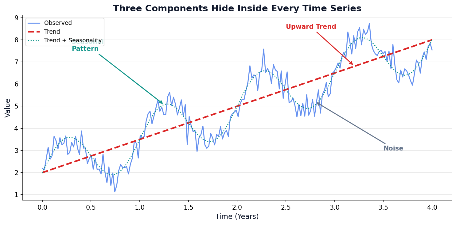
Four Components Hide Inside Every Series

Decomposition = splitting a series into its building blocks. Every time series is a mix of these four:

1. Trend (T)

The long-term direction — is the series going up, down, or flat over years?

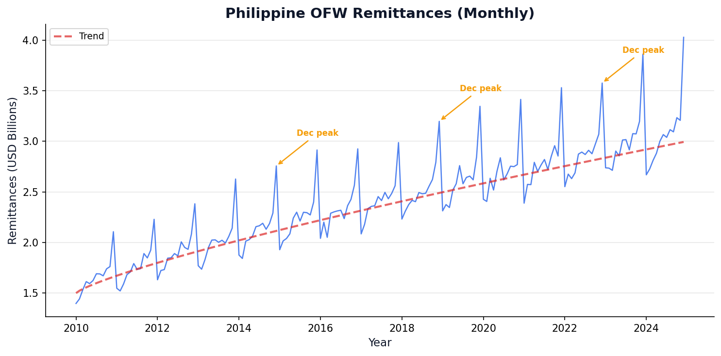
2. Seasonality (S)

Repeating patterns at fixed intervals — December peaks, weekend dips, summer surges.

3. Cyclical (C)

Rise and fall without fixed period — business cycles, economic booms/busts (years-long waves).

4. Residual / Noise (R)

Random leftover after removing the other three — unpredictable, ideally small.

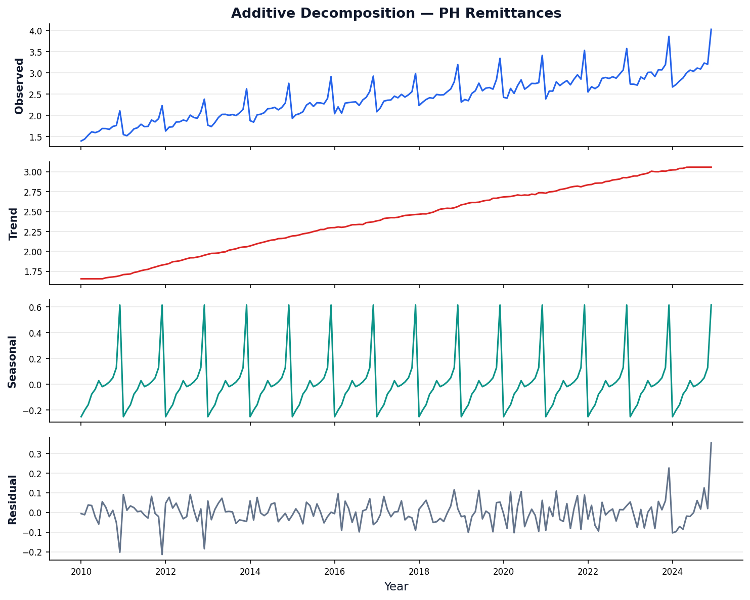
Additive

$Y_t = T_t + S_t + C_t + R_t$

Constant seasonal swing (+₱500M every Dec)

Multiplicative

$Y_t = T_t \times S_t \times C_t \times R_t$

Growing seasonal swing (+15% every Dec)

Time series with annotated trend, seasonal, cyclical, and noise components

Baseline Method

Naive Forecast: The Simplest Prediction

Rule: Tomorrow's value = today's value. That's it. The simplest possible forecast — and every other method must beat this to be useful.

Algorithm: Naive Forecast

for each time t:

ŷ_t = y_t−1

Golden Rule

"If your fancy model can't beat naive, throw it away." — Every forecasting textbook

The naive forecast always lags 1 step behind — it misses every move.

Part I · Fundamentals Interactive

Decomposition Reveals the Hidden Structure

Period:

Model:

What to Look For: In Additive mode, the Seasonal panel shows peaks of equal height throughout. The Residual should look like random noise near zero.

Model Comparison: Additive (Y=T+S+R): seasonal peaks stay the same size. Multiplicative (Y=T×S×R): peaks grow with the trend. Toggle between them — watch how the Seasonal and Residual panels change.

Part I · How It Works

Decomposition: Step by Step

Step 1: Extract Trend (T)

Smooth the series with a centered moving average of window = period.

T_t = \frac{1}{m}\sum_{j=-k}^{k} Y_{t+j}

For period $m$=12: average 12 months centered on each point. Removes seasonality, keeps only the long-term direction.

Step 2: Extract Seasonality (S)

Detrend first, then average all same-month values.

$D_t = Y_t - T_t$ (detrended) $S_{\text{month}} = \frac{1}{n}\sum D_t$ for all Jans, all Febs, …

Example: average all December detrended values → $S_{\text{Dec}}$ = +0.5 (always a peak).

Step 3: What's Left = Residual (R)

Subtract trend and seasonality from the original.

Additive: $R_t = Y_t - T_t - S_t$

Multiplicative: $R_t = \frac{Y_t}{T_t \times S_t}$

If the decomposition is good, R should look like random noise near zero (additive) or near 1 (multiplicative).

Decomposition: Observed, Trend, Seasonal, Residual panels

Reading the chart: Top panel = original data. Blue trend line rises over time. Green seasonal repeats every 12 months. Bottom residual should be random — if you see patterns there, the decomposition missed something.

Python code: see Appendix

Part I · Fundamentals

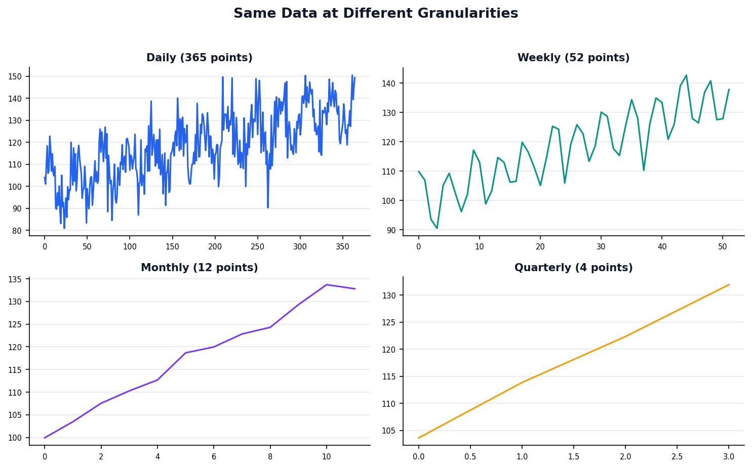
Resampling Changes the Granularity

Resampling means changing the time granularity — downsampling (daily → monthly) aggregates, upsampling (monthly → daily) interpolates.

Same data at daily, weekly, monthly, and quarterly granularity

Key Resample Codes

'W' = weekly 'M' = month-end 'Q' = quarter 'Y' = year

Code

weekly = df['sales'].resample('W').sum()
monthly = df['sales'].resample('M').mean()

Live Demo

Moving Average Explorer

Window: 5

Algorithm: Moving Average

1. for each time step t ≥ w:

forecast[t] = (y[t−w] + … + y[t−1]) / w

2. MAE = mean(|actual − forecast|)

Window=5: MAE=—

Part II

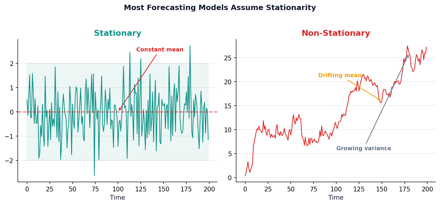
The Stationarity Requirement

Most forecasting models assume the future looks statistically like the past.

If the mean or variance drifts over time, predictions break down.

Part II · Stationarity

Forecasting Breaks When the Rules Keep Changing

Side-by-side stationary noise vs non-stationary random walk

Stationary Series

Stationary: statistical properties (mean, variance) stay constant over time — the rules don't change.

Constant mean over time
Constant variance over time
Covariance depends only on lag distance

Why It Matters

Non-stationary: mean or variance drifts over time — yesterday's patterns may not apply tomorrow.

ARIMA, exponential smoothing, and most forecasting models assume stationarity. Non-stationary data must be transformed first.

In plain English: If a stock price keeps going up forever, its average changes over time — that's non-stationary. Our models need stable rules to learn from.

Part II · Stationarity

The ADF Test

Hypothesis

H₀: Series has a unit root (non-stationary)
H₁: Series is stationary

p < 0.05 → Reject H₀ → Stationary ✓
p ≥ 0.05 → Non-stationary → difference & retest

ADF Equation

$\Delta y_t = \alpha + \beta y_{t-1} + \sum \gamma_i \Delta y_{t-i} + \varepsilon_t$

Test if $\beta = 0$ (shocks never fade)

if p < 0.05 → $\beta \neq 0$ → stationary

else → $y'_t = y_t - y_{t-1}$, retest

Unit root = past shocks never decay | p-value = probability under H₀

Python code: see Appendix

Part II · Stationarity

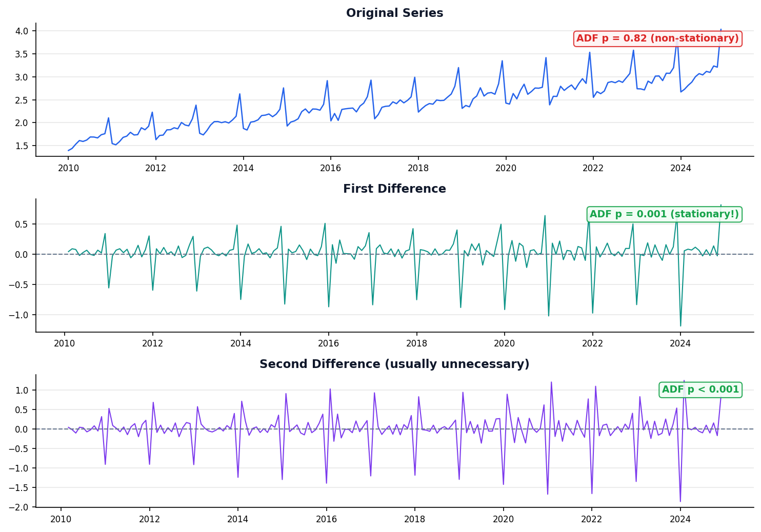
Differencing Removes the Trend

Three-panel differencing: original, first diff, second diff with ADF p-values

How It Works

Differencing (computing changes between consecutive values: Δy[t] = y[t] − y[t−1]) removes trend. Seasonal differencing (subtracting the value from one season ago: Δy[t] = y[t] − y[t−12]) removes seasonality.

diff_1 = df['sales'].diff() # 1st
diff_2 = df['sales'].diff().diff() # 2nd
seasonal = df['sales'].diff(12) # seasonal

Rule of Thumb

First differencing (d=1) fixes most trends. Second differencing (d=2) is rarely needed. Seasonal differencing handles calendar cycles.

Think of it as: Instead of asking "what's the price?", ask "how much did it change?" Changes are often more stable than levels.

Live Demo

Differencing Demo

Algorithm: Differencing for Stationarity

1. plot original → check for trend/seasonality

2. if trend: diff₁[t] = y[t] − y[t−1]

3. if seasonal: diff_s[t] = y[t] − y[t−period]

4. run ADF test → p < 0.05 = stationary ✓

5. now fit ARIMA on stationary residual

Knowledge Check

Stationarity Quiz

A PSEi closing price series has a clear upward trend over 5 years. What should you do before applying ARIMA?

A) Nothing, ARIMA handles trends

B) Apply first differencing

C) Remove all outliers first

D) Use a larger rolling window

Click to reveal answer

B) Apply first differencing

An upward trend means the series is non-stationary. First differencing (d=1) removes the linear trend and makes the series suitable for ARIMA.

Part III

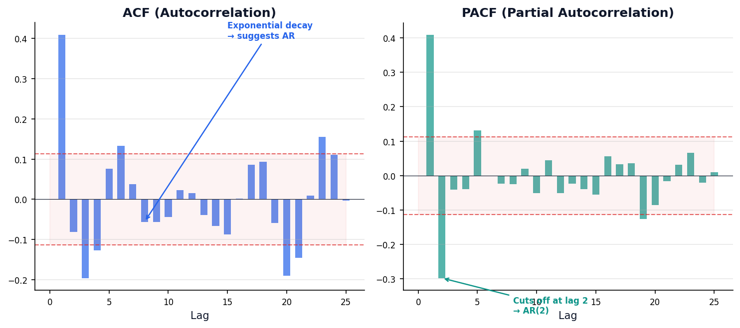
Reading the Autocorrelation Signature

ACF and PACF plots are the fingerprint of any time series — they tell you which model to use.

Part III · Autocorrelation

Past Values Predict Future Values

ACF (Autocorrelation Function)

Correlation between Y_t and Y_t-k at each lag k. Includes indirect effects through intermediate lags.

PACF (Partial Autocorrelation)

Direct correlation between Y_t and Y_t-k after removing effects of intervening lags.

ρ_k = Cov(Y_t, Y_t-k) / Var(Y_t)

Intuition: If sales were high last month, are they likely high this month too? Autocorrelation measures exactly this — how much the past predicts the future.

Definitions

Autocorrelation — how much a series correlates with its own past values
Lag — a delayed version of the series (lag-1 = last month, lag-12 = same month last year)
ACF (Autocorrelation Function) — shows correlation at every lag
PACF (Partial ACF) — shows direct correlation at each lag, removing intermediate effects

ACF showing exponential decay and PACF showing cutoff at lag 2 for AR(2) process

Part III · Autocorrelation

What Is Autoregression?

Autoregression (AR) is a regression where the predictors are the series' own past values — lagged versions of itself. An AR(p) model uses the last p observations to predict today.

ŷ_t = c + φ₁y_t−1 + φ₂y_t−2 + … + φ_py_t−p + ε_t

What

A linear model that regresses Y_t on its own lags. Each coefficient φ_i tells you exactly how much lag-i pulls on today.

Why

Captures temporal dependence cheaply. Simple, interpretable, and a strong baseline when past values carry real predictive signal.

When

PACF cuts off at lag p, the series is stationary (after differencing if needed), and no external regressors are required. Not for non-linear regimes.

OFW Remittance Intuition

This December's remittance is strongly predicted by last December's. Y_t and Y_t−12 correlate year after year — an AR term captures that persistence directly.

AR(1) — last month predicts this month (short memory).
AR(12) — same month last year predicts today (yearly cycle).
AR(p) — blend of the last p months.

Diagnostic Signal

A good AR fit leaves white-noise residuals — no pattern remains in ε_t. If residuals still autocorrelate, increase p or move to ARMA / ARIMA.

TL;DR AR(p) = "predict today from the last p yesterdays."

Part III · Autocorrelation

ACF/PACF Patterns Guide Model Choice

AR(p) (Autoregressive) — predict from p past values: ŷ_t = φ₁y_t−1 + φ₂y_t−2 + …
MA(q) (Moving Average) — predict from q past errors: ŷ_t = θ₁ε_t−1 + θ₂ε_t−2 + …

ACF Pattern	PACF Pattern	Model Suggested	Interpretation
Cuts off at lag q	Exponential decay	MA(q)	Past errors drive the series
Exponential decay	Cuts off at lag p	AR(p)	Past values drive the series
Exponential decay	Exponential decay	ARMA(p,q)	Both values and errors matter
Significant at lag s	Significant at lag s	Seasonal	Calendar-driven pattern

Part IV

Smoothing the Signal

Before forecasting, we need to separate signal from noise.

Smoothing techniques reveal underlying patterns by reducing random variation.

Part IV · Smoothing Interactive

Moving Averages Trade Detail for Clarity

Window A: 7

Window B: 30

Part IV · Smoothing Interactive

Exponential Smoothing Weights Recent Data More

Exponential Smoothing — a technique giving exponentially decreasing weights to older data. Recent observations matter more. SES (Simple Exponential Smoothing) uses one parameter α to balance between the latest data point and the previous smoothed value. α (alpha) — smoothing factor (0–1). Higher α = trusts recent data more. Lower α = smoother, slower to react.

S_t = 0.30 · Y_t + 0.70 · S_t-1

α = 0.30

The α Parameter

α → 0: Smooth, slow to react
α → 1: Reactive, follows every wiggle
Sweet spot: 0.2–0.3 for most business data

Live Demo

SES Step-Through Simulator

α = 0.30

t	Y_t	α·Y_t	(1-α)·S_t-1	S_t

Press Step to initialize S₁ = Y₁

Algorithm: Simple Exponential Smoothing

1. initialize: S₁ = Y₁

2. for t = 2, 3, …, n:

S_t = α · Y_t + (1−α) · S_t−1

3. forecast: ŷ_n+1 = S_n

Part IV · Smoothing

From SES to Holt-Winters: Handling Trend and Seasonality

SES

SimpleExpSmoothing(y)
.fit(smoothing_level=0.2)

Holt's (+ Trend)

Holt's method — extends SES to handle trend by adding a second smoothing equation for the slope.

ExponentialSmoothing(y,
trend='add').fit()

Holt-Winters (+ Season)

Holt-Winters — extends Holt's to handle trend + seasonality with a third equation for the seasonal component.

ExponentialSmoothing(y,
trend='add',
seasonal='add',
seasonal_periods=12).fit()

Live Demo

ARIMA Forecast Animator

Speed

Press Play or Step to begin.

Algorithm: ARIMA(2,1,0)

1. split → train (1–36) | test (37–48)

2. difference train data (d=1)

3. fit AR(p) on differenced data

4. forecast h steps + confidence intervals

5. compare vs actual → MAE

Big Picture

The Forecasting Ladder: Simple → Complex

Each method builds on the last. More complexity = more accuracy, but also harder to explain.

#	Method	Equation	MAE	Beats Naive?
1	Naive	ŷ_t = y_t−1	0.26	Baseline
2	Moving Avg	ŷ_t = mean(y_t−w:t)	0.43	No — lags behind
3	Diff + MA	MA on Δy + past	0.23	✓ Yes
4	SES (α=0.3)	S_t = αY_t + (1−α)S_t−1	0.21	✓ Yes
5	ARIMA(2,1,1)	φ₁y'_t−1 + φ₂y'_t−2 + θ₁ε_t−1	0.18	✓✓ Best classical
6	Prophet	g(t) + s(t) + h(t)	0.15	✓✓✓ Best overall

Session 1 Key Takeaways

Time series = ordered data where today depends on yesterday
Decomposition separates trend, seasonality, and noise
Stationarity is required for ARIMA — test with ADF, fix with differencing
ACF/PACF plots are your model selection guide
Exponential smoothing adapts to trend and seasonality

Next: Session 2 — Forecasting Methods (ARIMA, Prophet, Evaluation)

CMSC 178DA | Week 10 — Session 2

From Understanding to Prediction

ARIMA, Prophet & Evaluation

Department of Computer Science

University of the Philippines Cebu

Lecture 20: Forecasting & Evaluation

Jollibee Group Opens 700+ Stores Per Year

Every new location needs a multi-year sales forecast before opening day.

10,000+ outlets (all brands)

700+ new stores/year

5 yr strategic plan horizon

The tool they need? ARIMA and Prophet.

Agenda

Session 2 Objectives

ARIMA

Build ARIMA/SARIMA models and choose p, d, q parameters systematically.

Prophet

Use Meta Prophet for business forecasting with holidays and changepoints.

Evaluation

Measure forecast accuracy with MAE, RMSE, MAPE and proper temporal splits.

Part I

ARIMA: The Workhorse of Forecasting

Three ideas from Session 1 — autoregression, differencing, and moving average — combined into one powerful model.

Part I · ARIMA

What Is ARIMA?

ARIMA = AutoRegressive Integrated Moving Average — a single model that stitches together three Session 1 ideas into one framework, controlled by parameters (p, d, q).

What

AR(p) uses p past values, I(d) differences the series d times to remove trend, and MA(q) corrects using q past forecast errors. Parameters (p, d, q) say how much of each.

Why

One unified framework for trend + autocorrelation + shock-persistence. Well-understood theory, fast to fit on a laptop, and delivers built-in confidence intervals out of the box.

When

Univariate series with mild-to-moderate patterns, stationary after d differences, at least ~50 observations. Not for strong multi-seasonality (use SARIMA) or abrupt regime shifts (use Prophet).

Picking (p, d, q)

p → PACF cutoff · d → ADF test · q → ACF cutoff

Run ADF; difference until p-value < 0.05 → that's d.
Inspect PACF of differenced series → first lag that cuts off = p.
Inspect ACF of differenced series → first lag that cuts off = q.

Connect Back to Session 1

You already know each piece: AR from autocorrelation (Part III), I from differencing & the ADF test (Part II), and MA as a residual-correction mechanism. ARIMA just composes them.

TL;DR ARIMA(p, d, q) = AR + differencing + MA.

Part I · ARIMA

ARIMA Combines Three Ideas You Already Know

ARIMA = AutoRegressive Integrated Moving Average — the workhorse of classical time series forecasting. p = number of past values used (AR order) | d = number of times differenced | q = number of past errors used (MA order).

AR(p) — AutoRegressive

Past values predict future. PACF tells you p.

I(d) — Integrated

Differencing order for stationarity. ADF test tells you d.

MA(q) — Moving Average

Past errors correct future. ACF tells you q.

Part I · ARIMA

The ARIMA Equation in Plain English

Y_t = c + φ₁Y_t-1 + … + φ_pY_t-p + θ₁ε_t-1 + … + θ_qε_t-q + ε_t

In words: "Today's value = constant + weighted past values + weighted past errors + new shock."

Part I · ARIMA

Building ARIMA in Python

The statsmodels ARIMA class handles fitting, diagnostics, and forecasting.

Workflow

Choose p, d, q (from ACF/PACF or auto)
Fit model & check summary
Run diagnostics (residual plots)
Forecast with confidence intervals

Algorithm: Box-Jenkins Method

1. plot series → look for trend and seasonality

2. difference until ADF says stationary:

$y'_t = y_t - y_{t-1}$ ($d$ = number of diffs needed)

3. read ACF/PACF of differenced series:

PACF cuts off at lag $p$ → AR order | ACF cuts off at lag $q$ → MA order

4. fit the ARIMA equation:

$y'_t = c + \phi_1 y'_{t-1} + \phi_2 y'_{t-2} + \theta_1 \varepsilon_{t-1} + \varepsilon_t$

5. check residuals $\varepsilon_t \approx$ white noise? (no patterns left)

6. forecast: iterate forward CI = $\hat{y} \pm 1.96\,\sigma\sqrt{h}$

ARIMA(2,1,1) Model Summary

Parameter	Coeff	Std Err	Meaning
ar.L1	0.72	0.08	Strong positive from 1 month ago
ar.L2	-0.21	0.07	Mild correction from 2 months ago
ma.L1	-0.89	0.05	Strong error correction

AIC: 478.3 (lower = better)

Python code: see Appendix

Part I · ARIMA

Choosing p, d, q

Manual approach: 3 steps to find (p, d, q)

Automatic (pmdarima)

Searches all combinations of (p, d, q) and picks the one with the lowest AIC. No manual ACF/PACF reading needed.

AIC (Akaike Information Criterion) = fit quality − complexity penalty. Lower = better.

auto_arima Search Results

Model	AIC
ARIMA(0,1,0)	523.1
ARIMA(1,1,0)	498.4
ARIMA(2,1,0)	485.2
ARIMA(2,1,1)	478.3	← Best!
ARIMA(3,1,1)	479.8	worse

Which to use? Start with auto_arima for speed. Use Box-Jenkins manually when you want to understand why specific parameters were chosen.

Python code: see Appendix

Part I · ARIMA Interactive

Forecasting with Confidence Intervals

Forecast horizon — how many time steps into the future you're predicting. Longer = more uncertain. Confidence interval (CI) — a range (e.g., 95% CI) where the true value is likely to fall. CI widens with longer horizons.

Forecast Horizon: 30 steps

Why CIs Widen

Uncertainty compounds over time. Drag the slider to see how confidence bands grow with longer forecasts.

What this means: "We're 95% confident the true value will be between 8.2B and 9.8B." The band widens further into the future because uncertainty grows.

Python Equivalent

fc = results.get_forecast(30)
ci = fc.conf_int()

Part I · ARIMA

SARIMA Adds Seasonal Intelligence

SARIMA = Seasonal ARIMA. Adds seasonal AR, differencing, and MA on top of regular ARIMA. (P,D,Q,m): P = seasonal AR lags, D = seasonal differencing, Q = seasonal MA terms, m = period (12 = monthly).

ARIMA(p,d,q)(P,D,Q)_s

Seasonal Parameters

P: Seasonal AR order
D: Seasonal differencing
Q: Seasonal MA order
s: Seasonal period (12=monthly, 7=weekly)

Example: SARIMA(1,1,1)(1,1,1)₁₂

SARIMA(1,1,1)(1,1,1)₁₂ — 12-Month Forecast

Month	Forecast (B$)	95% CI
Jan	9.2	8.6 – 9.8
Mar	8.8	8.0 – 9.6
Jun	8.7	7.8 – 9.6
Sep	9.1	8.0 – 10.2	CI widens
Dec	10.1	8.8 – 11.4	Peak!

Key: The (1,1,1)₁₂ seasonal component captures the December remittance peak. CI grows from ±0.6 to ±1.3 further out.

Python code: see Appendix

Knowledge Check

ARIMA Quiz

Your ADF test gives p=0.03 after first differencing. PACF cuts off at lag 2 and ACF decays exponentially. What ARIMA order should you try?

A) ARIMA(0, 1, 2)

B) ARIMA(2, 1, 0)

C) ARIMA(1, 0, 1)

D) ARIMA(2, 0, 2)

Click to reveal answer

B) ARIMA(2, 1, 0)

PACF cutoff at 2 → p=2. One differencing needed (p=0.03 after) → d=1. ACF decays (doesn't cut off) → q=0. This is a pure AR(2) model on differenced data.

Part II

Prophet: Built for Business

Meta's open-source tool handles missing data, holidays, and changepoints automatically.

Designed for analysts who need good forecasts fast, not ARIMA experts.

Part II · Prophet

What Is Prophet?

Prophet is Meta's open-source additive decomposable forecasting model. Instead of requiring stationarity, it fits trend, seasonality, and holidays directly — and combines them with Bayesian parameter estimation.

y(t) = g(t) + s(t) + h(t) + ε_t

trend + seasonality + holidays + noise

What

Piecewise-linear trend g(t) with auto-detected changepoints, Fourier-series seasonality s(t), and user-defined holiday effects h(t), fit via Bayesian optimization (Stan/MCMC).

Why

Robust to missing data and outliers. Detects changepoints automatically. Interpretable components (trend / seasonality / holiday) you can plot separately. Analyst-friendly API — two columns: ds and y.

When

Business forecasting with strong calendar/holiday effects, messy real-world data, multiple seasonalities (daily + weekly + yearly), or when a non-specialist needs a good default quickly.

ARIMA vs Prophet — Pick the Right Tool

Property	ARIMA	Prophet
Needs stationarity?	Yes (differencing)	No
Handles missing data?	Poorly	Natively
Framework	Classical / MLE	Bayesian
Holidays & regressors	Manual (SARIMAX)	First-class
Best fit for	Clean, stationary	Messy, calendar-driven

Philippine Use Case

Monthly OFW remittances peak around December (Christmas sendings) and dip around Undas. Prophet models these as holiday effects and a piecewise trend without requiring us to difference the series first.

TL;DR Different tools, different jobs — we evaluate both in Part III.

Part II · Prophet

Prophet Solves Real Business Problems

Prophet — Meta's open-source library for business forecasting. Handles missing data, holidays, and trend changes automatically. Uses Fourier series (sine and cosine waves) to mathematically represent repeating seasonal patterns.

Missing Data

Handles gaps automatically — no imputation needed.

Outlier Robust

COVID-era spikes won't break your forecast.

Changepoints

Detects trend shifts automatically (e.g., policy changes).

Changepoint — a moment where the trend's growth rate shifts (e.g., new competitor enters market, policy change).

Holiday Effects

Add Christmas, Undas, or any custom event.

Part II · Prophet

Prophet Setup and Forecasting

Algorithm: Facebook Prophet

1. decompose into 3 learnable components:

$y(t) = g(t) + s(t) + h(t) + \varepsilon_t$

$g(t)$ = piecewise linear trend with auto-detected changepoints

$s(t) = \sum_{n=1}^{N}\left[a_n \cos\!\left(\frac{2\pi nt}{P}\right) + b_n \sin\!\left(\frac{2\pi nt}{P}\right)\right]$ (Fourier)

$h(t)$ = indicator function for holidays (Christmas, Undas, …)

2. fit all parameters via Bayesian optimization (Stan/MCMC)

3. forecast with uncertainty: sample from posterior distribution

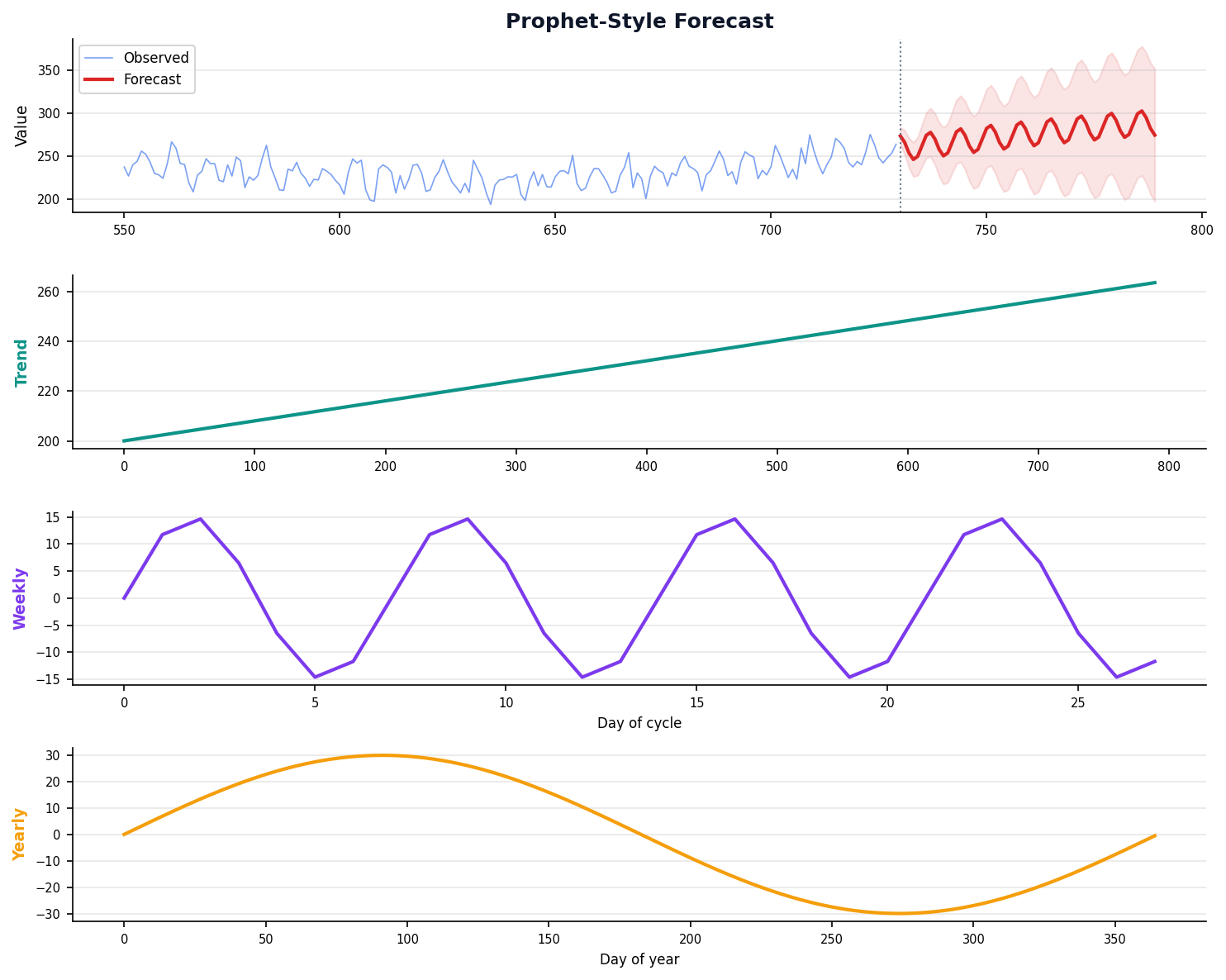
Output: DataFrame with ds (date), yhat (prediction), yhat_lower/upper (95% CI). Use model.plot_components() for trend + seasonality breakdown.

Python code: see Appendix

Part II · Prophet

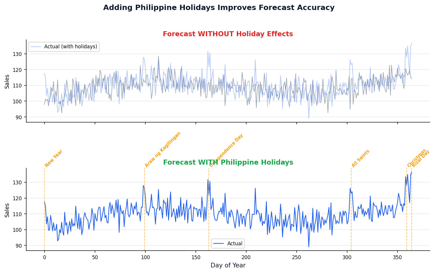
Philippine Holidays Make Forecasts Smarter

Forecast comparison with and without Philippine holiday effects

Code

ph_holidays = pd.DataFrame({
  'holiday': 'ph_holiday',
  'ds': ['2024-12-25', '2024-11-01',
        '2024-06-12', '2024-04-09'],
  'lower_window': 0,
  'upper_window': 1
})
model = Prophet(holidays=ph_holidays)

Window Parameters

lower_window: days before the holiday affected. upper_window: days after. E.g., Christmas shopping starts early: lower_window=-7.

Part III

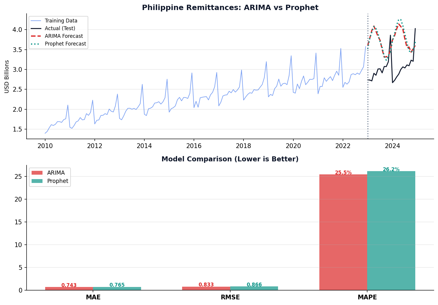
Measuring Forecast Quality

A forecast without an error estimate is just a guess.

This section covers metrics, temporal splits, and model comparison.

Part III · Evaluation

Four Metrics Every Analyst Must Know

Metric	Formula	Interpretation	When to Use
MAE	mean(\|y − ŷ\|)	Average absolute error in original units	General purpose
RMSE	√mean((y − ŷ)²)	Penalizes large errors more	When big misses are costly
MAPE	mean(\|y − ŷ\|/y) × 100	Percentage error — scale-free	Stakeholder reports
MASE	MAE / naive_MAE	<1 means better than naive forecast	Comparing across datasets

TL;DR Use MAPE for business stakeholders. Use RMSE when large errors are costly.

RMSE (Root Mean Squared Error) — like MAE but penalizes big errors more heavily (squares them first, then takes the root).
MAPE (Mean Absolute Percentage Error) — error as a percentage; easy to explain ("our forecast is off by 5% on average").
MASE (Mean Absolute Scaled Error) — compares your model's error to naive forecast error. MASE < 1 means you beat naive.

Part III · Evaluation

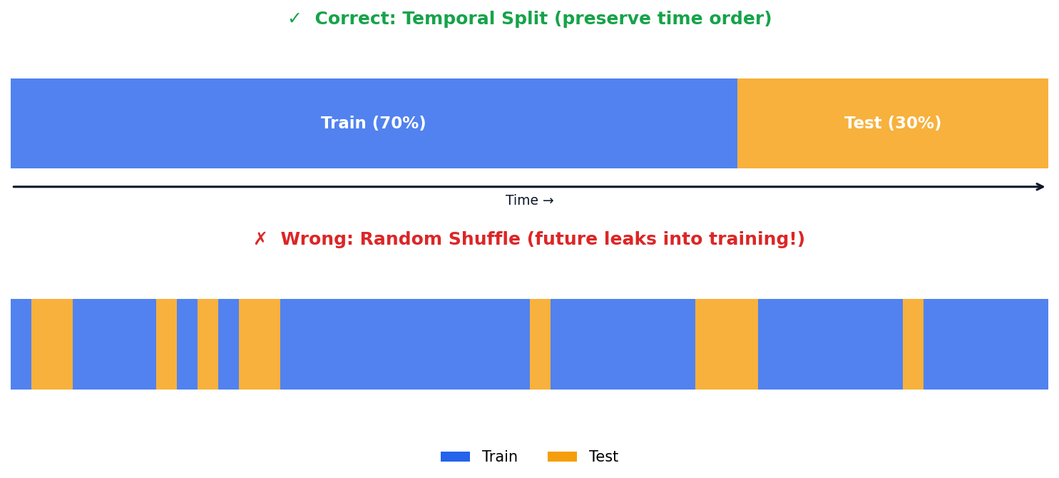
Time Series Train-Test Split: Never Shuffle

Temporal split — split by TIME (train on past, test on future). Never shuffle time series data! White noise — a series of completely random values with no pattern (mean=0, constant variance). Good residuals look like white noise.

Correct temporal split vs wrong random shuffle comparison

Code

# Preserve time order!
train = df['sales'][:-30]
test = df['sales'][-30:]

# Never use: train_test_split(shuffle=True)

Why No Shuffling?

Random shuffling lets future data leak into training. Your model "sees the future" and metrics look artificially good.

Part III · Capstone

Philippine Remittances: Complete Forecasting Pipeline

Complete pipeline comparing ARIMA vs Prophet on Philippine remittance data

Pipeline Steps

Load BSP data & set datetime index
Decompose to understand components
Test stationarity & difference
Fit ARIMA + Prophet on training data
Compare MAPE on held-out test set

Key Insight

Neither model is universally better. ARIMA excels on clean, stationary data. Prophet handles messy, real-world data with holidays and gaps.

Live Demo

Method Showdown Race

#	Method	MAE	vs Naive

Current Method

1. select a forecasting method

2. train on months 1–36

3. forecast months 37–48

4. compute MAE = mean(|actual − forecast|)

Resources

Keep Learning: Free Courses & Datasets

These free resources go deeper into every topic we covered today.

Kaggle: Time Series

Free 6-lesson micro-course with hands-on notebooks.

Linear Regression with Time Series
Trend & Seasonality
Time Series as Features (lags, rolling)
Hybrid Models (linear + XGBoost)
Forecasting with ML

kaggle.com/learn/time-series

TF Developer Certificate

Course 4: Sequences, Time Series & Prediction (Coursera).

Week 1: Patterns & Metrics
Week 2: DNN for Forecasting
Week 3: RNN & LSTM
Week 4: Conv1D + Real-World Data

Video from this course included in slide 5

Philippine Datasets

Practice with real PH data for your lab project.

BSP — OFW remittances (monthly)
PSA OpenSTAT — GDP, inflation, trade
PAGASA — rainfall, temperature
DOH — disease surveillance

Links on the course portal

Session 2 Key Takeaways

ARIMA(p,d,q) = AR + differencing + MA in one model
Use ACF/PACF or auto_arima to choose parameters
SARIMA adds seasonal (P,D,Q)_s for periodic data
Prophet is ideal for business forecasting with holidays and missing data
Always use temporal train-test splits, never random shuffle
MAPE is the most intuitive metric for business stakeholders

Lab 10: Time Series Forecasting Project

Forecast a Philippine economic indicator. Compare ARIMA vs Prophet. Present results to "management."

Python Code Reference

Complete runnable code for every algorithm.
Copy-paste into your Jupyter notebook.

Appendix

Decomposition Code

What This Does

Splits a time series into trend, seasonal, and residual components using statsmodels.

Key Parameters

model: 'additive' or 'multiplicative'
period: seasonal cycle length (12 for monthly)

import pandas as pd
from statsmodels.tsa.seasonal import seasonal_decompose
import matplotlib.pyplot as plt

df = pd.read_csv('bsp_remittances.csv',
                  parse_dates=['date'])
df.set_index('date', inplace=True)

decomp = seasonal_decompose(
    df['remittances_usd'],
    model='additive',  # or 'multiplicative'
    period=12           # monthly seasonality
)

decomp.plot()
plt.tight_layout()
plt.show()

Appendix

ADF Test Code

What This Does

Tests whether a time series is stationary using the Augmented Dickey-Fuller test. p < 0.05 means stationary.

from statsmodels.tsa.stattools import adfuller

result = adfuller(df['remittances_usd'])

print(f'ADF Statistic: {result[0]:.4f}')
print(f'p-value:       {result[1]:.4f}')

if result[1] < 0.05:
    print("Stationary! Ready to model.")
else:
    print("Non-stationary. Apply diff.")
    # Apply differencing
    df_diff = df['remittances_usd'].diff().dropna()
    result2 = adfuller(df_diff)
    print(f'After diff - p: {result2[1]:.4f}')

Appendix

ARIMA Code

What This Does

Fits an ARIMA(p,d,q) model and generates forecasts with confidence intervals.

order=(p, d, q)

p: AR lags
d: differencing order
q: MA terms

from statsmodels.tsa.arima.model import ARIMA

# Fit model
# order=(p, d, q) = (2 AR, 1 diff, 1 MA)
model = ARIMA(df['sales'], order=(2, 1, 1))
results = model.fit()

# Model summary
print(results.summary())

# Diagnostic plots (residuals)
results.plot_diagnostics(figsize=(12, 8))

# Forecast 30 steps ahead
forecast = results.get_forecast(steps=30)
mean = forecast.predicted_mean
ci = forecast.conf_int()  # 95% CI

Appendix

auto_arima Code

What This Does

Automatically searches for the best (p,d,q) by comparing AIC scores. No manual ACF/PACF reading needed.

from pmdarima import auto_arima

auto_model = auto_arima(
    df['sales'],
    start_p=0, max_p=5,
    start_q=0, max_q=5,
    d=None,        # auto-detect d
    seasonal=False,
    trace=True     # show AIC comparisons
)

print(auto_model.summary())
# Best model: ARIMA(2,1,1) AIC=478.3

Appendix

SARIMA Code

What This Does

Extends ARIMA with seasonal components. The seasonal_order=(P,D,Q,m) adds monthly patterns.

seasonal_order=(P, D, Q, m)

P,D,Q: seasonal AR, diff, MA
m=12: monthly cycle

from statsmodels.tsa.statespace.sarimax import SARIMAX

model = SARIMAX(
    df['remittances_usd'],
    order=(1, 1, 1),
    seasonal_order=(1, 1, 1, 12)
    # P=1, D=1, Q=1, period=12 months
)
results = model.fit(disp=False)

# Forecast next 12 months
forecast = results.forecast(steps=12)
print(forecast)

Appendix

Prophet Code

What This Does

Meta's Prophet handles trends, seasonality, and holidays automatically. Requires columns named 'ds' (date) and 'y' (value).

from prophet import Prophet

# Prepare data (must have 'ds' and 'y')
df_p = df.reset_index()
df_p.columns = ['ds', 'y']

# Fit model
model = Prophet(
    yearly_seasonality=True,
    weekly_seasonality=True,
    daily_seasonality=False
)
model.fit(df_p)

# Forecast
future = model.make_future_dataframe(periods=30)
forecast = model.predict(future)

# Visualize
model.plot(forecast)
model.plot_components(forecast)

Predicting the Future with Data

Every Quarter, $8.9 Billion Flows into the Philippines

Session 1 Objectives

Components

Stationarity

Smoothing

Meet Our Data: OFW Remittances

Three Patterns to Spot

What Makes Time Unique

Common Time Series Patterns

0:00 — Trend

0:30 — Seasonality

1:30 — Autocorrelation

3:00 — Non-Stationary

Time Series Data Has Memory

Key Characteristics

Four Components Hide Inside Every Series

1. Trend (T)

2. Seasonality (S)

3. Cyclical (C)

4. Residual / Noise (R)

Additive

Multiplicative

Naive Forecast: The Simplest Prediction

Golden Rule

Decomposition Reveals the Hidden Structure

Decomposition: Step by Step

Step 1: Extract Trend (T)

Step 2: Extract Seasonality (S)

Step 3: What's Left = Residual (R)

Resampling Changes the Granularity

Key Resample Codes

Code

Moving Average Explorer

The Stationarity Requirement

Forecasting Breaks When the Rules Keep Changing

Stationary Series

Why It Matters

The ADF Test

Hypothesis

Differencing Removes the Trend

How It Works

Rule of Thumb

Differencing Demo

Stationarity Quiz

Reading the Autocorrelation Signature

Past Values Predict Future Values

ACF (Autocorrelation Function)

PACF (Partial Autocorrelation)

Definitions

What Is Autoregression?

What

Why

When

OFW Remittance Intuition

Diagnostic Signal

ACF/PACF Patterns Guide Model Choice

Code

Smoothing the Signal

Moving Averages Trade Detail for Clarity

Python Equivalent

Window Size Tradeoff

Exponential Smoothing Weights Recent Data More

The α Parameter

SES Step-Through Simulator

From SES to Holt-Winters: Handling Trend and Seasonality

SES

Holt's (+ Trend)

Holt-Winters (+ Season)

ARIMA Forecast Animator

The Forecasting Ladder: Simple → Complex

Session 1 Key Takeaways

From Understanding to Prediction

Jollibee Group Opens 700+ Stores Per Year

Session 2 Objectives

ARIMA

Prophet

Evaluation

ARIMA: The Workhorse of Forecasting

What Is ARIMA?

SARIMA(1,1,1)(1,1,1)₁₂ — 12-Month Forecast