Mining Meaning
from Text
From raw words to actionable insights
Department of Computer Science
University of the Philippines Cebu
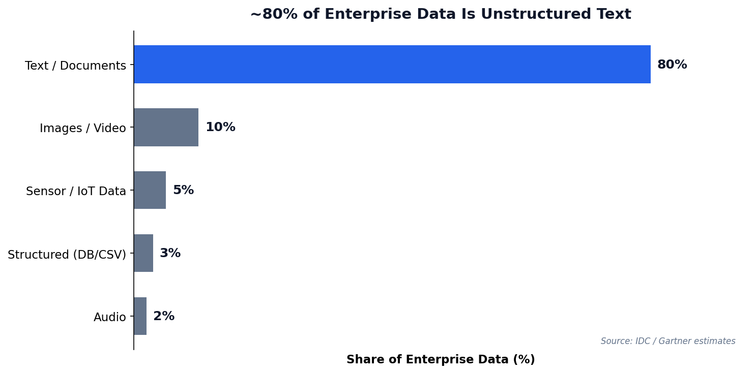
"80% of enterprise data is unstructured — and much of it is text."
"The limits of my language mean the limits of my world."
— Ludwig Wittgenstein, 1921
Today: how to teach machines to understand text — and how to use that power responsibly.
When NLP Goes Wrong
Amazon's AI Recruiting Tool (2018)
Reuters exclusive report, October 2018
Amazon trained an NLP model on 10 years of resumes to automate hiring. The model learned to penalize resumes containing the word "women's" (e.g., "women's chess club captain") and downgrade graduates of all-women's colleges.
Why? The training data was 10 years of mostly male hires. The model learned that "male" patterns predicted success. Amazon scrapped the entire program.
Text analytics is powerful — but the data you train on encodes the biases of the world that produced it.
Session 1 Objectives
Text Preprocessing
Tokenize, clean, and normalize raw text into analysis-ready tokens.
Vectorization
Convert words into numbers using Bag of Words and TF-IDF representations.
Sentiment & Topics
Classify polarity with sentiment analysis and discover themes with LDA topic modeling.
Meet Our Data: PH Social Media
Throughout this session, we will preprocess, vectorize, and analyze these posts. They represent real patterns in Philippine social media data.
The Challenge
Code-switching (Taglish), informal spelling, emojis, and sarcasm make PH social media data uniquely difficult for NLP tools built for English.
| # | Platform | Post | Sentiment |
|---|---|---|---|
| 1 | "Grabe ang bilis ng GCash today! Love it" | Positive | |
| 2 | "Ang bagal ng internet dito sa probinsya" | Negative | |
| 3 | "Just tried the new Jollibee menu, it's okay naman" | Neutral | |
| 4 | "Sobrang init ngayon, parang oven ang Cebu" | Negative | |
| 5 | "Congrats sa mga bagong graduates! Proud kami!" | Positive | |
| 6 | "The new MRT extension is a game changer" | Positive | |
| 7 | "Nag-update na ba kayo ng PhilSys ID? Hassle amp" | Negative | |
| 8 | "May pasok ba bukas? Walang announcement eh" | Neutral |
Turning Noise
Into Signal
Natural language is messy. Preprocessing cleans, normalizes, and tokenizes text before any model can learn.
Why Text Analytics?
Unstructured text data is everywhere — and growing faster than any other data type.
Text Data Sources
- Customer reviews & feedback
- Social media posts & comments
- Support tickets & emails
- News articles & reports
- Survey open-ended responses
70 Years of Text Analytics
Why this history matters
Each era didn't replace the previous — they layered. Today's production pipelines mix all of them: regex preprocessing (1960s), TF-IDF retrieval (1990s), and LLM generation (2020s).
Where this lecture sits
We focus on the Classical ML era (★) — BoW, TF-IDF, VADER, TextBlob. These are the foundations every modern system still relies on for cheap, interpretable, fast text features.
Three Paradigms, Side by Side
| Paradigm | Era | Core Idea | Strengths | Weaknesses |
|---|---|---|---|---|
| Symbolic / Rule-based ELIZA, hand-rules |
1950s–80s | Encode language as explicit grammars and dictionaries | Transparent, debuggable, no training data needed | Brittle; doesn't generalize; rules explode in complexity |
| Statistical / Classical ML ★ BoW, TF-IDF, VADER, LDA, SVM |
1990s–2010s | Count word frequencies, learn weights from labeled corpora | Fast, cheap, interpretable; works on small data | Loses word order & meaning; lexicons are language-bound (e.g. no Filipino) |
| Neural / Transformers BERT, GPT, Claude, Llama |
2017–today | Learn contextual representations from billions of tokens via self-attention | State-of-the-art on every benchmark; multilingual; multimodal | Expensive; opaque; hallucinates; data & compute hungry |
The "embarrassingly effective" baseline
A 1990s-style TF-IDF + logistic regression often beats a fine-tuned BERT for short, domain-specific text classification — at 1/1000th the compute cost. Always benchmark the simple thing first.
Today's stack is hybrid
Modern RAG systems use TF-IDF/BM25 (Era 3) to retrieve documents, then an LLM (Era 7) to generate the answer. Old methods aren't dead — they're load-bearing for the new ones.
The Preprocessing Pipeline
Raw text needs cleaning before any algorithm can use it. Each step transforms the data into a more useful form.
Preprocessing in Python
NLTK Library
The Natural Language Toolkit provides tokenizers, stemmers, lemmatizers, and stopword lists for 20+ languages.
Key Functions
word_tokenize()— split into wordsstopwords.words()— common words listWordNetLemmatizer()— dictionary lookup
Caveat: POS Tagging
WordNet defaults to noun POS — “running” stays as-is. Pass pos='v' for verb lemmatization to get “run”.
['dog', 'running', 'fast']
["the","dogs","are","running","fast"] → drop "the","are" → lemmatize → 3 tokens
Preprocessing Step by Step
Watch a real Taglish tweet get transformed through each pipeline stage.
| Step | Operation | Result |
|---|---|---|
| Raw | — | Grabe ang ganda ng new GCash update!! 💯🔥 #fintech |
| 1. Lowercase | .lower() | grabe ang ganda ng new gcash update!! 💯🔥 #fintech |
| 2. Tokenize | word_tokenize() | ['grabe', 'ang', 'ganda', 'ng', 'new', 'gcash', 'update', '!', '!', '💯', '🔥', '#', 'fintech'] |
| 3. Remove stopwords + non-alpha | isalpha() + stopword filter | ['grabe', 'ganda', 'new', 'gcash', 'update', 'fintech'] |
| 4. Lemmatize | WordNetLemmatizer() | ['grabe', 'ganda', 'new', 'gcash', 'update', 'fintech'] |
Notice: Filipino words survive
"grabe" and "ganda" pass through because they are not in the English stopword list. This is why Taglish text needs combined stopword lists.
Emojis & hashtags removed
The isalpha() filter strips emojis, punctuation, and the # symbol. Some NLP pipelines keep emojis for sentiment analysis.
Text Preprocessing Simulator
| Step | Operation | Result |
|---|
Stemming vs. Lemmatization
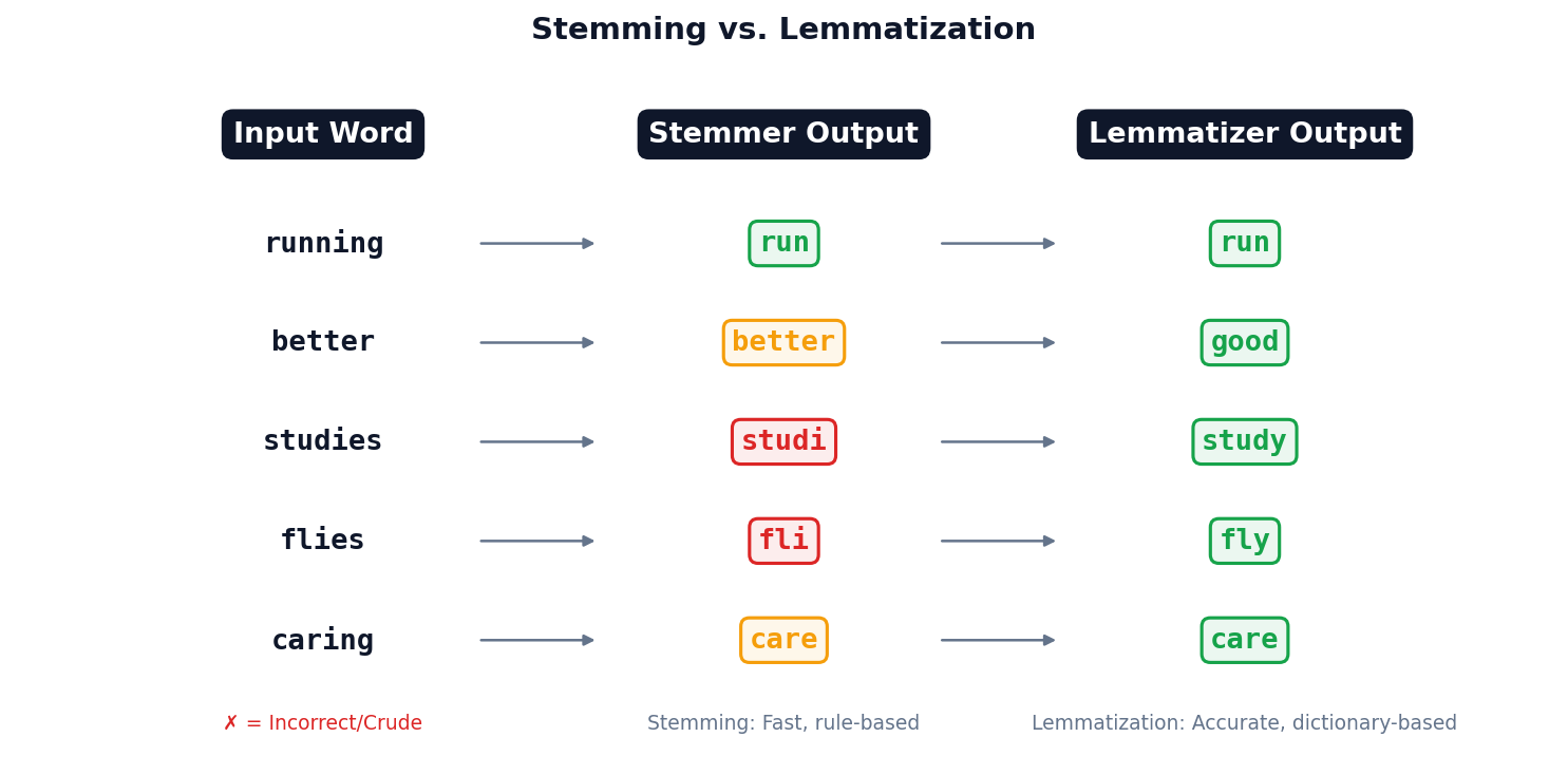
Rule-based suffix stripping. “studies” → “studi” (not a real word). Use when speed matters more than accuracy.
Dictionary-based lookup. “studies” → “study”. Slower but produces valid words. Preferred for analytics.
Making Words
Countable
Machines need numbers, not words. Bag of Words and TF-IDF convert text into vector space.
From Words to Numbers
The Core Problem
Algorithms work on numbers, not text. We need a way to convert "The food was good" into a vector a computer can crunch.
The Idea
Treat each document as an unordered "bag" of words. Build a vocabulary, then count occurrences.
Bag of Words in Practice
The simplest text representation: count how many times each word appears.
Limitations
- Loses word order entirely
- Common words dominate the counts
- High-dimensional, sparse matrices
The Problem with Just Counting Words
The Issue
In Bag of Words, "the" appears 50 times in a document — looks like the most "important" word. But it appears in every document. Useless signal.
The Insight
A word is truly important when it's:
- Frequent in this document (the topic)
- Rare across all documents (distinguishing)
TF-IDF: The Formula, Step by Step
① Term Frequency (TF)
"How frequent is term t in document d?" Normalize by doc length so long docs don't dominate.
② Inverse Document Frequency (IDF)
"How rare is t across all N documents?" Use log so it grows slowly with N.
③ Multiply Them
High TF × High IDF = important word for this doc.
TF-IDF in Python
Key Parameters
max_features— limit vocabulary sizemin_df— ignore very rare termsmax_df— ignore very common termsngram_range— include bigrams
TF-IDF = TF × log(N/df). Words that are frequent in a document but rare across the corpus get the highest score.
TF-IDF by Hand
3 mini-documents. Compute TF-IDF for the word "gcash" in Doc 1.
Documents
- "gcash users love the new gcash savings feature" (7 words)
- "gcash reports strong quarterly growth numbers today" (7 words)
- "bitcoin prices surge amid global market rally today" (8 words)
Formulas
$\text{TF}(t,d) = \frac{\text{count of } t \text{ in } d}{|d|}$
$\text{IDF}(t) = \log\!\left(\frac{N}{df_t}\right)$
$\text{TF-IDF} = \text{TF} \times \text{IDF}$
| Step | Calculation | Value |
|---|---|---|
| TF("gcash", Doc 1) | 2 occurrences / 7 words | $2/7 = 0.286$ |
| df("gcash") | Appears in Doc 1, Doc 2 | 2 documents |
| IDF("gcash") | $\log(3/2)$ | $0.176$ |
| TF-IDF | $0.286 \times 0.176$ | $\mathbf{0.050}$ |
Interpretation
"gcash" is moderately important in Doc 1: it appears often (high TF) but also in another doc (lowers IDF). A word like "savings" (only in Doc 1) would score higher.
TF-IDF Scores Across Documents
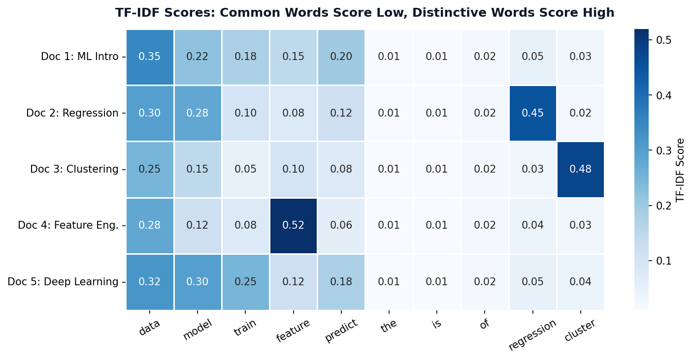
Low Scores (Blue)
Stopwords like “the”, “is”, “of” appear everywhere → low IDF → near-zero TF-IDF.
High Scores (Dark Blue)
Distinctive terms like “regression” or “cluster” appear in few documents → high IDF → high TF-IDF.
TF-IDF Ranking Challenge
Instructions (5 min, pairs)
Given these 3 PH news headlines from a corpus of 100 articles:
- "GCash launches new savings feature for Filipino users"
- "BSP raises interest rates amid inflation concerns"
- "Filipino fintech GCash reports 86M registered users"
Rank these words by likely TF-IDF score (highest first):
savings Filipino the GCash inflation reports
Hint: Think about which words are frequent in their document but rare across all 100 articles.
TF-IDF Explorer
Which term has the HIGHEST TF-IDF score?
✓ Correct: B) “analytics”
High TF (appears 5 times in those docs) × high IDF (only 2/100 docs) = highest TF-IDF. Terms A, C, D have low IDF because they appear in most documents.
Reading Between
the Lines
Sentiment analysis classifies text polarity — positive, negative, or neutral — using lexicons or machine learning.
Three Approaches to Sentiment Analysis

Lexicon-Based
VADER, SentiWordNet. Fast, no training. Best for social media text.
ML-Based
Naive Bayes, SVM. Needs labeled data. Custom domain accuracy.
Pre-trained
BERT, RoBERTa. State-of-the-art. Requires GPU compute.
VADER Sentiment
What is VADER?
Valence Aware Dictionary and sEntiment Reasoner. Rule-based, tuned for social media text.
Compound Score
Ranges from -1 (most negative) to +1 (most positive). Threshold: >0.05 positive, <-0.05 negative.
VADER Doesn't Speak Filipino
"Grabe ang ganda!"
compound = 0.0
NEUTRAL — VADER has no Filipino lexicon
"This is absolutely wonderful!"
compound = 0.87
POSITIVE — VADER recognizes English intensifiers
Same meaning, different language, completely different result.
This is why off-the-shelf NLP tools fail for Philippine social media data.
Inside TextBlob's Two Scores
① Polarity (−1 to +1)
Average word polarity from the Pattern lexicon, weighted by intensifiers.
$p_w$ = word polarity, $m_w$ = intensifier modifier (e.g., "very" = 1.3×)
② Subjectivity (0 to 1)
Ratio of opinion-bearing words to all scored words.
TextBlob Sentiment
Two Dimensions
- Polarity: -1 (negative) to +1 (positive)
- Subjectivity: 0 (factual) to 1 (opinionated)
Per-Sentence Analysis
Analyze each sentence separately for mixed-sentiment texts like product reviews.
Philippine Social Media Sentiment
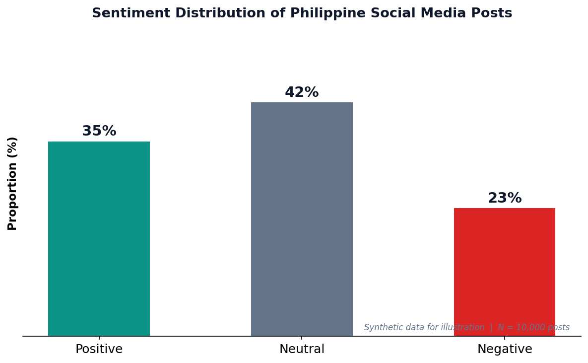
Philippine Social Media
With 98M internet users and 95M social media accounts (DataReportal 2026), the Philippines is one of the most active countries online. Sentiment analysis helps brands, government, and researchers understand public opinion.
Caveat
VADER was designed for English text. Filipino/Taglish posts may need custom lexicons or translated models for accurate results.
Sentiment Analyzer
ML Sentiment Pipeline
TF-IDF + Naive Bayes
A simple yet effective pipeline: vectorize text with TF-IDF, then classify with Naive Bayes (a classifier that assumes features are independent given the class — "naive" because this is rarely true, yet it works surprisingly well). The Multinomial variant models word counts/frequencies, making it ideal for text.
When to Use ML-Based
- Domain-specific language (medical, legal)
- You have labeled training data
- Lexicon approaches underperform
Discovering
Hidden Themes
LDA topic modeling reveals latent topics. NER extracts named entities. Word clouds visualize term frequencies.
LDA Topic Modeling
Quick Reminder
Supervised = labeled data, model learns input→output mapping. Unsupervised = no labels, model discovers structure on its own. LDA is unsupervised.
Latent Dirichlet Allocation
Unsupervised algorithm that discovers hidden topics in a collection of documents.
Key Assumptions
- Documents are mixtures of topics
- Topics are distributions over words
- You choose number of topics (k)
- Input must be word counts, not TF-IDF
Handling Filipino Text
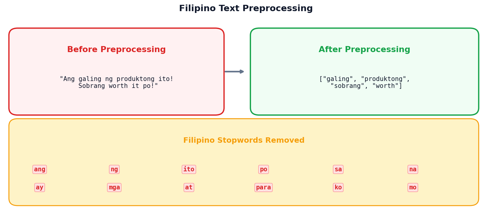
Filipino Stopwords
Standard NLTK stopwords are English-only. For Taglish text, combine English + Filipino stopwords: ang, ng, sa, na, ay, mga, at, para, ko, mo.
Code-Switching Challenge
Filipino social media often mixes English and Filipino (“Taglish”). Both stopword lists must be applied for effective preprocessing.
Method Comparison: Text Analytics Toolkit
| Method | Input | Output | Best For | PH Limitation |
|---|---|---|---|---|
| Bag of Words | Raw text | Word count vectors | Simple classification, baselines | Ignores Taglish word order |
| TF-IDF | Raw text | Weighted term vectors | Search, document similarity | No Filipino IDF corpora available |
| VADER | English text | Polarity scores (-1 to +1) | Social media, informal text | Zero Filipino coverage |
| TextBlob | English text | Polarity + subjectivity | Quick sentiment + objectivity | English-only lexicon |
| ML Pipeline | Labeled data | Predicted classes | Domain-specific sentiment | Needs Filipino labeled dataset |
| LDA | Word counts | Topic distributions | Theme discovery, exploration | Filipino stopwords needed |
Key Takeaway
No single method works for everything. The right tool depends on your data, language, and goal.
PH Context
Every method has a Philippine limitation — mostly around Filipino/Taglish language support. This is an active research area.
LDA Topic Discovery
Session 1: Key Takeaways
- Preprocessing is critical — lowercase, tokenize, remove stopwords, lemmatize
- TF-IDF weights important terms higher than common words
- Sentiment analysis has three approaches: lexicon, ML, and pre-trained
- LDA discovers hidden topics in document collections
- Filipino text needs custom stopwords and Taglish handling
Next: Analytics at Scale & Ethics
Big data tools, privacy regulations, algorithmic bias, and responsible AI.
Scale, Privacy
& Fairness
When data gets big, ethics must get bigger
Department of Computer Science
University of the Philippines Cebu
"With great data comes great responsibility."
The Philippine Data Explosion
86M+
GCash registered users
98M
Internet users in PH
95M
Social media accounts
Who protects this data?
Session 2 Objectives
Big Data Tools
When pandas isn’t enough: Spark, cloud platforms, and the 5 Vs of big data.
Privacy & Compliance
GDPR, Philippine DPA (RA 10173), anonymization, and consent requirements.
Bias & Fairness
Sources of algorithmic bias, fairness metrics, mitigation strategies, and responsible AI.
When pandas
Is Not Enough
Big data demands distributed computing. Learn when and why to scale beyond a single machine.
The 5 Vs of Big Data
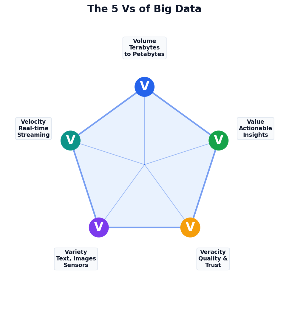
Beyond Just Size
Big data isn’t only about volume. Velocity (speed), variety (types), veracity (quality), and value (insights) all matter.
Philippine Example
GCash: 13M daily transactions (velocity) across payments, loans, investments (variety) with fraud detection needs (veracity).
When Do You Need Big Data Tools?
- Data fits in memory (<16 GB)
- Processing is one-time, ad-hoc
- Simple aggregations / filters
- pandas + SQL handles it fine
- Data exceeds single machine memory
- Processing must be parallelized
- Real-time streaming is required
- ML at scale (millions of records)
Most analytics tasks (<10 GB) don’t need Spark. Use the simplest tool that works.
Apache Spark
Distributed Computing
- In-memory processing (up to 100× faster than MapReduce in memory; typically 3–10× in practice)
- Supports Python (PySpark), SQL, Scala, R
- MLlib for machine learning at scale
When to Choose Spark
Datasets >100 GB, iterative ML algorithms, streaming data, or when a single machine can’t keep up.
Cloud Analytics Platforms
| Platform | Service | Strength | Pricing Model |
|---|---|---|---|
| AWS | Redshift, Athena, EMR | Most comprehensive ecosystem | Per-query or provisioned |
| GCP | BigQuery | Serverless SQL at scale | Per-TB scanned |
| Azure | Synapse Analytics | Enterprise integration (Office 365) | DWU-based |
Your dataset is 500 MB of CSV files.
Which tool should you use?
✓ Correct: B) pandas on your laptop
500 MB fits comfortably in memory. No need for distributed computing overhead. Use the simplest tool that works!
The Right to
Be Forgotten
Privacy regulations like GDPR and the Philippine DPA define how data can be collected, used, and stored.
Data Privacy Regulation Timeline
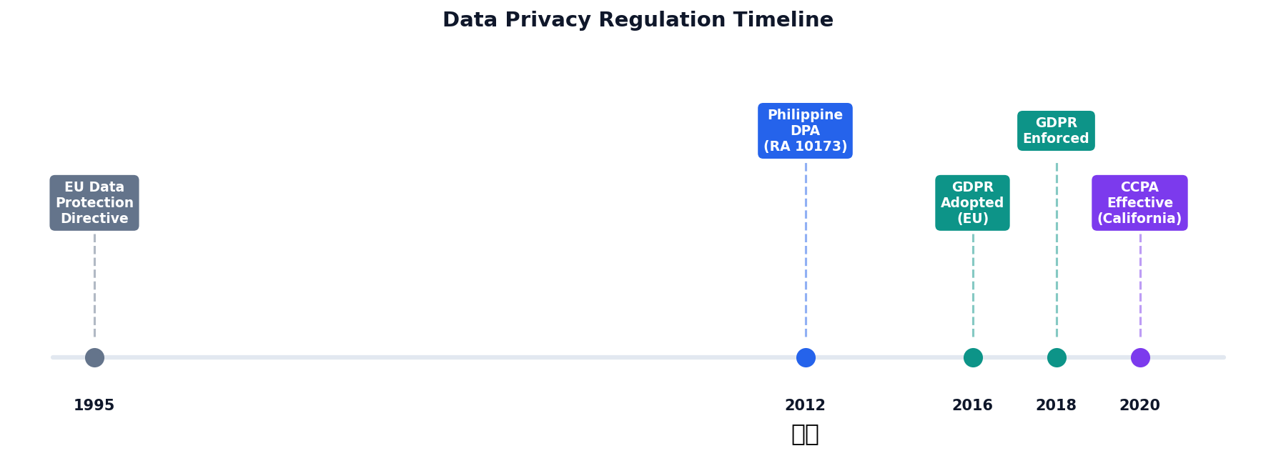
GDPR (EU, 2018)
Gold standard for privacy. Right to deletion, data portability, fines up to 4% of global revenue.
Philippine DPA (2012)
RA 10173. Enforced by NPC. Consent, purpose limitation, breach notification within 72 hours.
CCPA (California, enacted 2018, effective 2020)
Consumer right to know, delete, and opt-out of data sales. Applies to large businesses.
Philippine Data Privacy Act (RA 10173)
Consent
Freely given, specific, and informed
Purpose
Use only for stated purpose
Minimization
Collect only what’s needed
Accuracy
Keep data up to date
Retention
Delete when no longer needed
National Privacy Commission (NPC)
The NPC enforces the DPA, investigates breaches, and can impose fines and imprisonment for violations.
Breach Notification
Organizations must notify the NPC and affected individuals within 72 hours of discovering a personal data breach.
Anonymization Techniques
| Technique | Description | Example |
|---|---|---|
| Masking | Hide partial data | “Juan D.” |
| Generalization | Broaden categories | Age 25 → “20–30” |
| Suppression | Remove identifiers | Remove SSN column |
| Noise Addition | Add random values | Salary ± 5% |
| K-Anonymity | Ensure k similar records | 5+ with same quasi-identifiers |
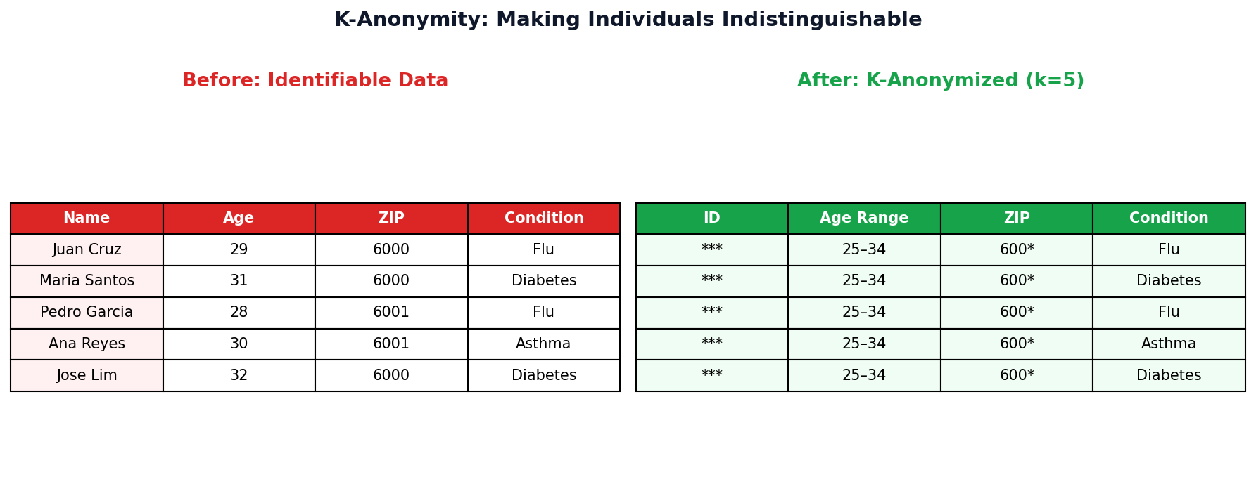
K-Anonymity
Definition
A dataset satisfies k-anonymity if every combination of quasi-identifiers (attributes that alone are harmless but together can identify someone, e.g. age, ZIP, gender) matches at least k other records.
Why k ≥ 5?
With k=5, an attacker can narrow a person down to at most 1-in-5 records — not enough to re-identify.
K-Anonymity Step by Step (k=3)
Before: Identifiable
| Name | Age | ZIP | Disease |
|---|---|---|---|
| Maria Santos | 28 | 6000 | Flu |
| Juan Cruz | 29 | 6001 | Diabetes |
| Ana Reyes | 27 | 6000 | Flu |
| Pedro Lim | 42 | 6045 | Asthma |
| Rosa Garcia | 44 | 6046 | Flu |
| Carlo Tan | 43 | 6045 | Asthma |
After: k=3 Anonymized
| Name | Age | ZIP | Disease |
|---|---|---|---|
| *** | 25-30 | 600* | Flu |
| *** | 25-30 | 600* | Diabetes |
| *** | 25-30 | 600* | Flu |
| *** | 40-45 | 604* | Asthma |
| *** | 40-45 | 604* | Flu |
| *** | 40-45 | 604* | Asthma |
1. Suppress
Remove direct identifiers (Name → ***).
2. Generalize
Age: exact → range. ZIP: last digit → *.
3. Verify k=3
Each (Age, ZIP) combo has ≥3 rows. An attacker can narrow to at most 1 in 3.
When Algorithms
Discriminate
Bias in data becomes bias in decisions. Understanding sources and metrics is the first step toward fairness.
Four Sources of Algorithmic Bias
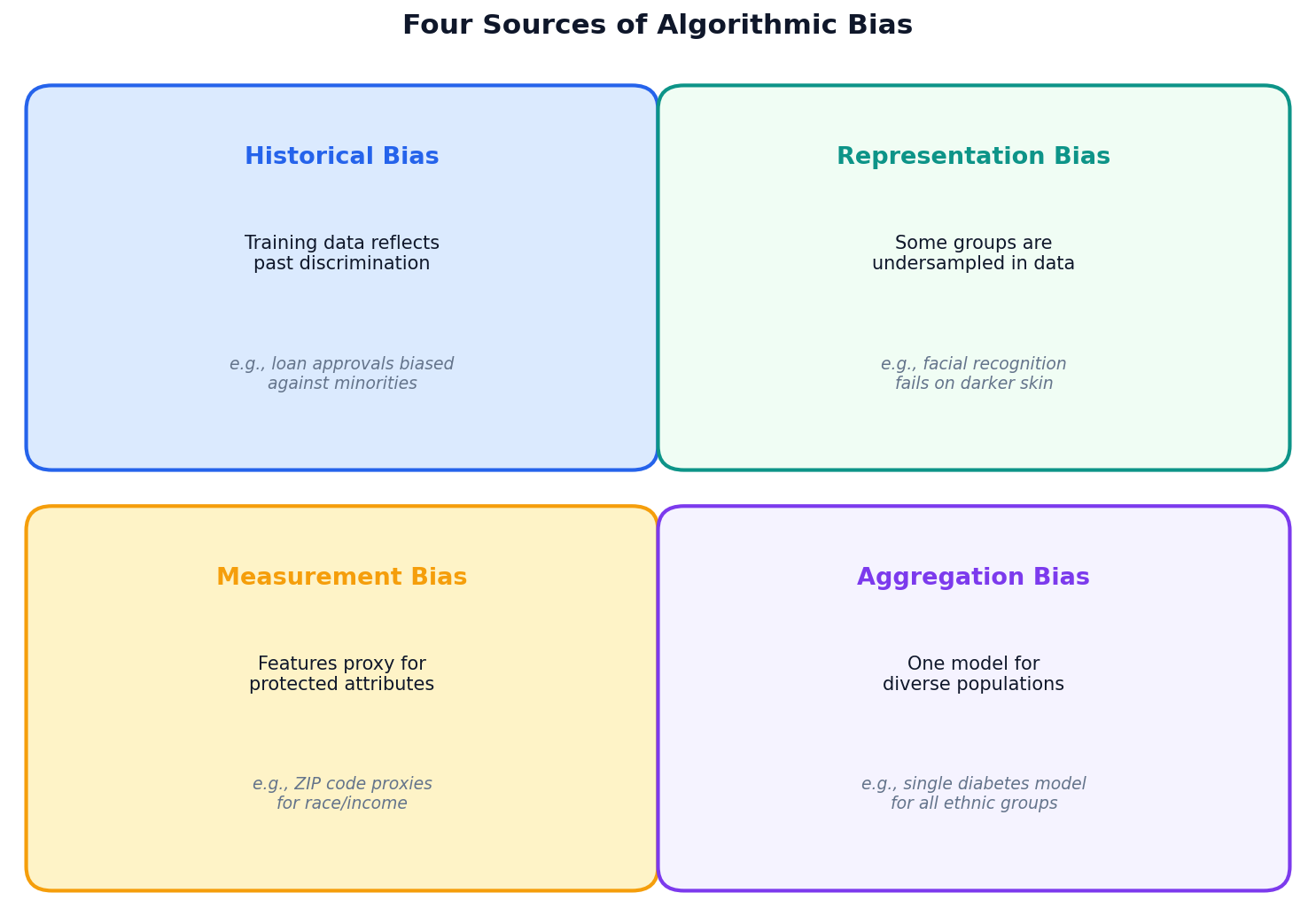
Key Insight
Bias is rarely intentional. It enters through the data, the features, and the modeling choices we make — often invisibly.
Systemic Impact
Biased models deployed at scale can affect millions: loans denied, jobs not offered, sentences lengthened.
Real-World Bias Failures
COMPAS (Criminal Justice)
Predicted recidivism risk for sentencing. ProPublica found it produced higher false positive rates for Black defendants than white defendants. Used in real sentencing decisions.
Amazon Hiring Tool (HR)
Trained on 10 years of (mostly male) hiring data. The model learned to penalize resumes containing the word “women’s”. Amazon scrapped the entire program.
Detecting Bias
Confusion Matrix
A 2x2 table comparing predicted vs. actual labels. Four cells: TP (correctly flagged), FP (wrongly flagged), TN (correctly cleared), FN (wrongly missed).
Check Metrics by Group
Split predictions by demographic and compare error rates. Significant differences indicate disparate impact (when a model's error rates differ substantially across protected groups).
What to Look For
- Unequal false positive rates (FPR)
- Unequal false negative rates (FNR)
- Different accuracy across groups
FPR by Gender: Is This Fair?
A GCash credit model flags applicants as "high risk." Let's compute FPR by gender.
Male Applicants
FP = 3, TN = 47 → $\text{FPR}_{\text{male}} = \frac{3}{3+47} = 0.06$ (6%)
Female Applicants
FP = 8, TN = 42 → $\text{FPR}_{\text{female}} = \frac{8}{8+42} = 0.16$ (16%)
Female FPR is 2.7x higher
Women are incorrectly flagged as "high risk" almost 3 times more often than men.
What This Means
16% of creditworthy women are wrongly denied vs. only 6% of men. Same model, same threshold, very different outcomes.
The Fix?
Adjust thresholds per group (post-processing), rebalance training data (pre-processing), or add fairness constraints (in-processing).
"Fair" Means Different Things
There's No Single Definition
"Treat people equally" sounds simple. But equally how? Equal treatment? Equal outcomes? Equal error rates? Each is a different mathematical formula — and they're incompatible.
Kleinberg's Impossibility (2017)
Mathematically proven: you cannot satisfy all common fairness metrics simultaneously (unless your model is perfect, which it never is).
Fairness Metrics
| Metric | Definition | When to Use | Example |
|---|---|---|---|
| Demographic Parity | Equal positive prediction rates across groups | Hiring, lending | Same loan approval rate for all demographics |
| Equalized Odds | Equal TPR and FPR across groups | Criminal justice | Same error rates regardless of race |
| Calibration | Equal precision across groups | Medical diagnosis | 70% confidence means 70% correct for all groups |
Impossibility Theorem
You cannot satisfy all fairness metrics simultaneously (Chouldechova, 2017). Choose based on your domain’s values.
Context Matters
Criminal justice prioritizes equalized odds (equal error rates). Lending prioritizes demographic parity (equal access).
Disparate Error Rates Across Groups
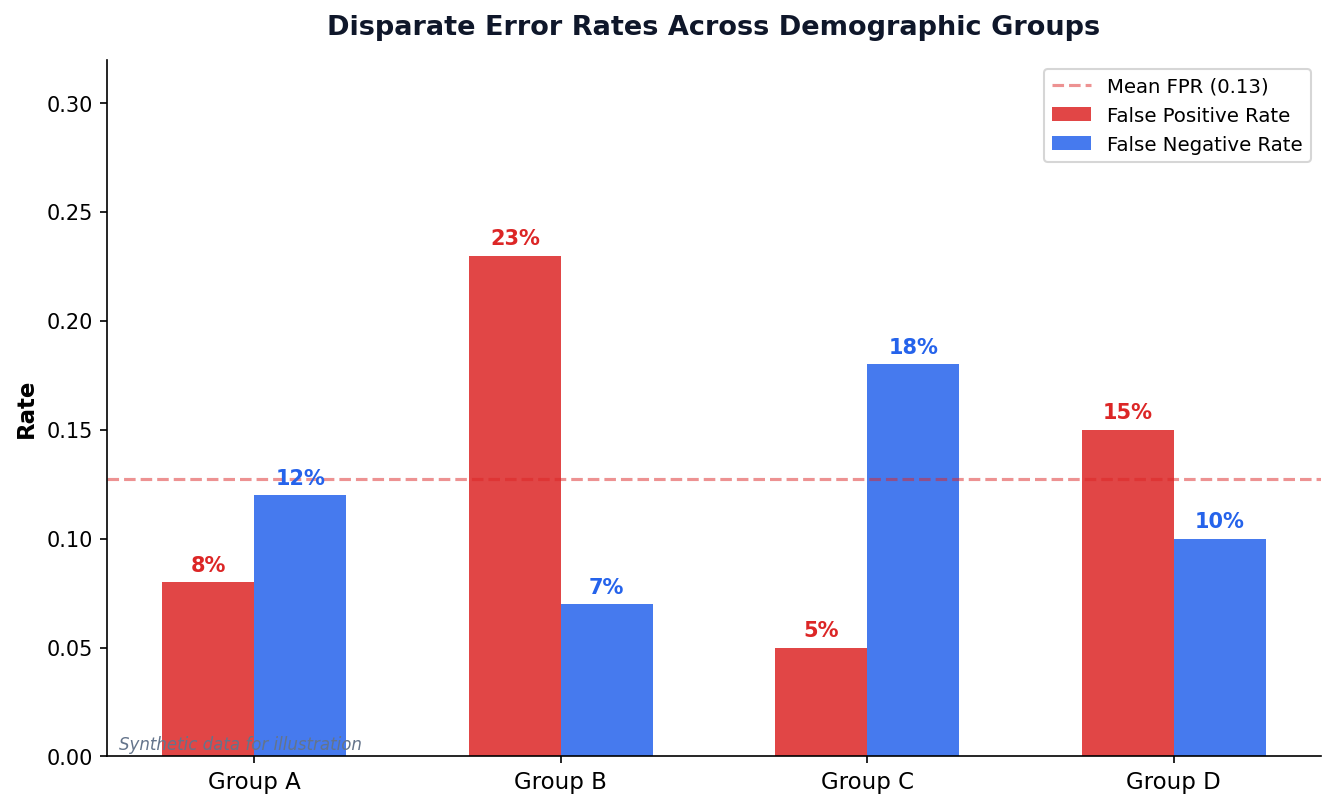
Group B: 3× Higher FPR
Group B is falsely flagged at 23% vs. 5–8% for others. This is the kind of disparity COMPAS exhibited.
Trade-off: FPR vs FNR
Lowering FPR for Group B may raise FNR. The question is: which error is more harmful in your context?
Bias in Practice
Activity 2: Ethical Dilemma (4 min, pairs)
Your team builds a GCash credit scoring model. After auditing, you discover the false positive rate for female applicants is 2x higher than for males — women are incorrectly denied credit twice as often.
- What stage of mitigation would you apply (pre-, in-, or post-processing)?
- What specific technique would you use?
- Who should be notified about this finding?
Discussion: Facial Recognition in PH Malls (4 min)
Several Philippine malls have deployed facial recognition for security. Commercial systems have higher error rates for darker skin tones and women.
- Should facial recognition be allowed in PH malls? Under what conditions?
- Who benefits? Who is harmed?
- What safeguards would you require under RA 10173?
Bias Detector Simulator
| ID | Gender | Income | Actual | Predicted |
|---|
Mitigating Bias: Three Stages
Pre-processing
Fix the data before training. Rebalance datasets, remove proxy features, use synthetic oversampling (SMOTE — generates synthetic minority-class samples by interpolating between existing ones).
In-processing
Fix the algorithm. Add fairness constraints to the loss function, use adversarial debiasing (train an adversary to detect demographic info from predictions — penalize the model if it leaks), or fair representation learning.
Post-processing
Fix the output. Adjust decision thresholds per group, calibrate probabilities, or audit and correct predictions.
Building AI That
Serves Everyone
Explainability, accountability, and ethics must be designed in — not bolted on after deployment.
The Black Box Problem
The Issue
Deep models & ensembles can have millions of parameters. Even the people who built them can't easily explain a single prediction.
High-Stakes Settings
- "Why was my loan denied?"
- "Why did this AI recommend prison?"
- "Why was my resume rejected?"
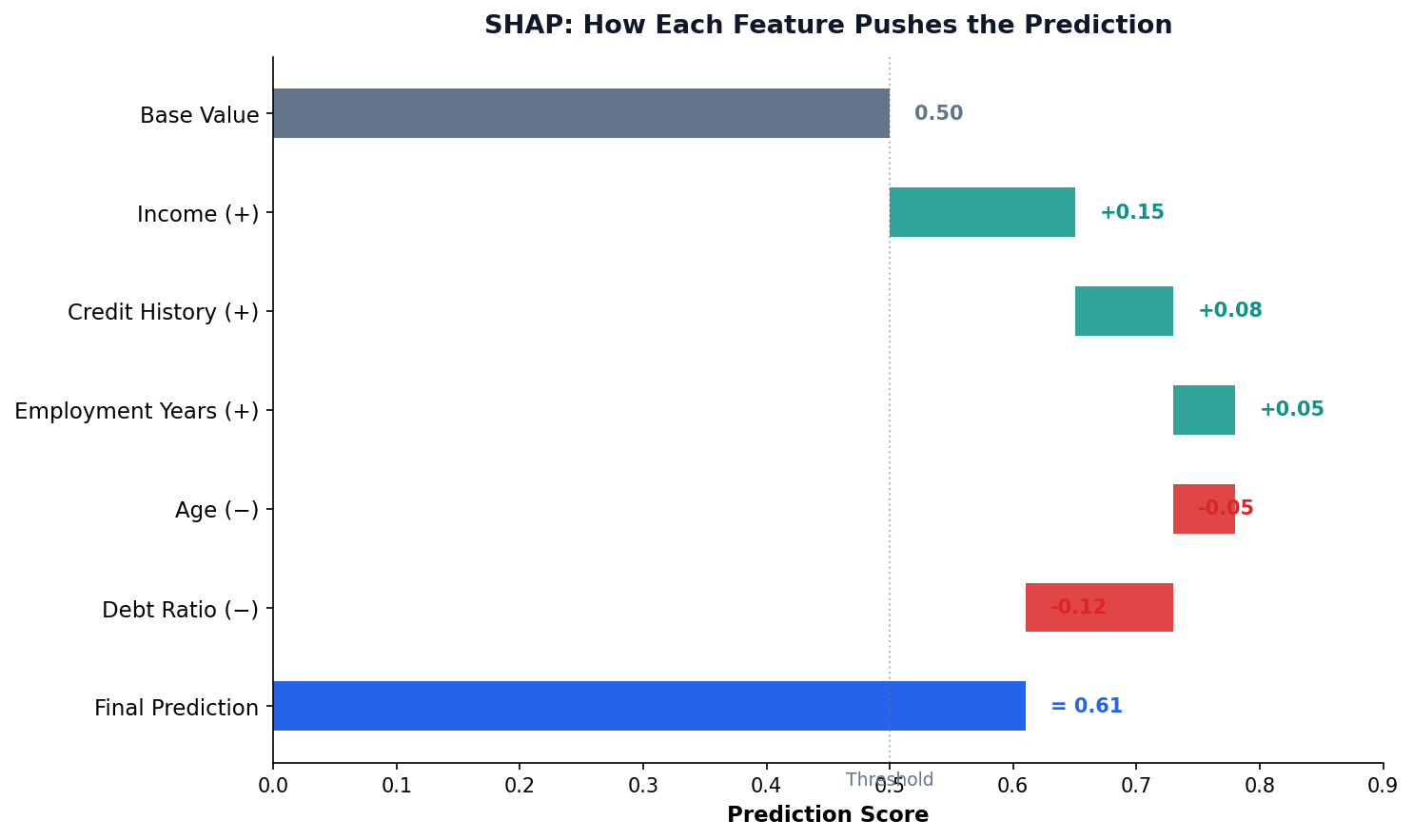
SHAP: Fair Credit from Game Theory
Origin: Shapley (1953)
Cooperative game theory: how to fairly divide rewards among teammates whose individual contributions are entangled.
The Formula
$\phi_i$ = SHAP value for feature $i$ $F$ = all features $S$ = subset without $i$
Average the marginal contribution of $i$ across all possible orderings in which it could be added.
LIME: Local Linear Approximation
Core Idea (Ribeiro et al., 2016)
The complex model $f$ is non-linear globally — but in a small neighborhood around any point $x$, you can fit a simple linear model $g$ that explains it.
The Optimization
$g$ = simple model (linear) $\pi_x$ = neighborhood weights (closer = more weight) $\Omega$ = simplicity penalty
Explainability: SHAP & LIME
Why Explainability?
- GDPR right to “meaningful information about the logic involved” (Art. 13–15)
- Build trust with stakeholders
- Debug model errors and biases
- Regulatory compliance
Key Tools
- SHAP: Shapley values — fair attribution of each feature’s contribution
- LIME: Local explanations via interpretable surrogate models
From FAT to FATE(S): An Evolving Framework
2018: FAT
ACM launches FAccT conference. Three pillars: Fairness, Accountability, Transparency. Reaction to ProPublica's COMPAS exposé and other public failures.
2018: FATE (+ Ethics)
Microsoft Research adds Ethics — recognizing that legal compliance ≠ moral correctness. The right question: should we even build this?
2020+: FATE(S) (+ Safety)
Columbia DSI adds Safety — preventing harm to users and bystanders, especially as models get deployed in safety-critical settings (healthcare, autonomous vehicles).
FATE(S) is Not a Checklist — Pillars Conflict
Maximizing one pillar can hurt another. Real engineering means choosing trade-offs, not satisfying all five.
Fairness ⟷ Accuracy
Example: A loan model has 92% accuracy overall — but enforcing demographic parity drops it to 87%.
Some accuracy must be "spent" on fairness. (Kleinberg 2017)
Transparency ⟷ Privacy
Example: Showing how the model uses your medical history is transparent — but reveals sensitive personal data.
Full transparency can leak protected information.
Safety ⟷ Helpfulness
Example: A chatbot that refuses medical questions is "safe" but useless for the user actually asking.
Over-restriction = unhelpful. Under-restriction = harm.
Accountability ⟷ Speed
Example: Auditing every prediction creates a paper trail (good!) — but slows deployment from minutes to weeks.
Bureaucracy is the cost of accountability.
Ethics ⟷ Profit
Example: "Should we train on user data we collected?" — legal under TOS but ethically dubious without clear consent.
Just because it's legal doesn't mean it's right.
The Right Mindset
FATE(S) is a compass, not a checklist. Engineers make explicit trade-offs and document the reasoning.
Document what you sacrificed and why.
The FATE(S) Framework
Fairness
Equal treatment across demographic groups
Accountability
Clear ownership and responsibility for outcomes
Transparency
Explainable decisions and open processes
Ethics
Consider societal impact and human values
Safety
Prevent harm to users and communities
Not a Checklist
FATE is a continuous practice, not a one-time audit. Models must be monitored after deployment for drift and emerging bias.
Origins
Core framework: FATE (Microsoft Research). The “S” for Safety added by Columbia DSI. Also see the ACM FAccT conference on Fairness, Accountability, and Transparency.
Ethics Challenges in the Philippines
GCash Credit Scoring
How do you score creditworthiness for informal economy workers with no traditional credit history? What biases might emerge?
DOH Disease Prediction
Rural areas have less data, worse connectivity. Models trained on urban data may fail in provinces where they’re needed most.
Facial Recognition
Commercial facial recognition has higher error rates for darker skin tones and women. Deployed in Philippine malls and airports.
Social Media Monitoring
With 95M accounts, social media surveillance raises privacy concerns. Where is the line between public safety and privacy?
Opportunity
Build AI that works for Filipinos, not just Western populations. Use local data, local context, and local values to create systems that serve everyone equitably.
Session 2: Key Takeaways
- Big data tools are needed only when scale demands it — don’t over-engineer
- Philippine DPA (RA 10173) governs data privacy; know its five principles
- Algorithmic bias enters through data, features, and modeling choices
- Fairness metrics help quantify bias — but you can’t satisfy all of them
- Responsible AI (FATE) requires continuous attention, not one-time audits
Lab 11: Bias Audit Project
Audit a model for bias, calculate fairness metrics, and propose mitigation strategies.
Sentiment Math Deep-Dive
VADER and TextBlob both look like simple lexicon lookups, but their published algorithms specify exact constants. These three slides show the formulas behind the high-level rules.
The Compound Score Formula
Step 1 — Sum modified valences
$v_i'$ = lexicon valence after CAPS, punctuation, booster, and negation modifiers.
Step 2 — Squash to [−1, +1]
Softsign-style squashing. As $|x| \to \infty$, compound → ±1. At $x=0$, slope is $1/\sqrt{15} \approx 0.258$.
The Magic Numbers Behind "Apply Modifiers"
① Punctuation
Each `!` (up to 4) adds +0.292 in the same direction. Question marks add +0.18 each (up to 3).
② ALL CAPS
Only triggers when sentence is mixed case. "This is GREAT" > "this is great"; "THIS IS GREAT" ≈ "this is great".
③ Degree Adverbs (boosters)
$B$ = ±0.293 (very/barely). Distance damping $s_1{=}1.0,\ s_2{=}0.95,\ s_3{=}0.9$ over the previous 3 tokens.
④ Negation
If not / never / n't is within 3 tokens behind. Not −1: "not great" softens to negative without flipping fully.
⑤ Contrastive "but"
Pre-"but" valences shrink, post-"but" valences amplify — matches the human reading that the second clause carries the speaker's true position. "Food was great BUT service was terrible" → net negative.
Corrected Worked Example
What Slide 18a glossed over
The earlier slide showed 0.8 × 1.3 = 1.04 → clipped to 1.0. In real Pattern code, clipping happens after the weighted average — not in the numerator.
Polarity (faithful)
For the example: $\dfrac{0.8 \cdot 1.3}{1.3} = 0.8$. The 1.3× modifier cancels in numerator and denominator when there's only one assessment.
Subjectivity (unweighted!)
Plain average over $N$ scored adjectives — no modifier weighting.