Introduction to Digital Image Processing
CMSC 178IP - Module 01
Noel Jeffrey Pinton
Department of Computer Science
University of the Philippines Cebu
What is Digital Image Processing?
Input
- Digital image(s)
- 2D array of pixel values
Output
- Enhanced image
- Extracted information
- Measurements or features
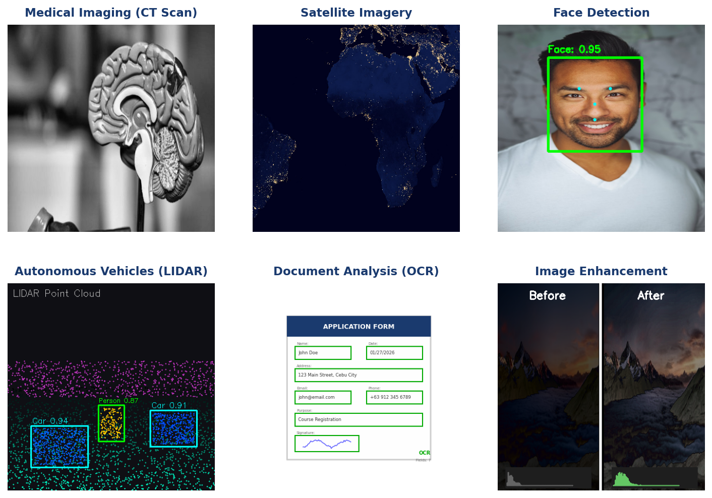
Real-World Applications
Where is DIP Used?
- Medical Imaging: CT scans, MRI, X-rays
- Satellite & Remote Sensing: Weather, agriculture, mapping
- Autonomous Vehicles: Object detection, lane recognition
- Biometrics: Face recognition, fingerprint analysis
- Social Media: Filters, enhancement, compression
Learning Objectives
By the end of this module, you will:
- Explain how digital images are represented as 2D arrays
- Describe the processes of sampling and quantization
- Distinguish between binary, grayscale, and color images
- Understand RGB and HSV color models
- Calculate memory requirements for different image types
Image as a 2D Function
Continuous
- $x, y \in \mathbb{R}$
- Infinite precision
- Real-world scene
Discrete
- $m \in \{0, ..., M-1\}$
- $n \in \{0, ..., N-1\}$
- Finite pixels
Knowledge Check
Think About It
What does f(x,y) represent in image processing?
Click the blurred area to reveal the answer
From Continuous to Discrete
Image Coordinate System
Standard Convention
- Origin: Top-left corner at (0, 0)
- x-axis: Increases to the right (columns)
- y-axis: Increases downward (rows)

Spatial Sampling
Higher Sampling Rate
- More pixels
- More detail preserved
- Larger file size
Lower Sampling Rate
- Fewer pixels
- Loss of detail
- Aliasing artifacts
Knowledge Check
Think About It
What happens if we sample below the Nyquist rate?
Click the blurred area to reveal the answer
Effect of Sampling Rate

Observations
- 512×512: Full detail (262,144 pixels)
- 128×128: Some detail loss (16,384 pixels)
- 32×32: Heavy pixelation (1,024 pixels)
Spatial Resolution

Common Resolutions
- VGA: 640 × 480 (307,200 pixels)
- Full HD: 1920 × 1080 (2.07 megapixels)
- 4K: 3840 × 2160 (8.29 megapixels)
Intensity Quantization
Common Bit Depths
- 1-bit: 2 levels (binary)
- 4-bit: 16 levels
- 8-bit: 256 levels
- 16-bit: 65,536 levels
Effects
- Fewer levels → visible banding
- More levels → smoother gradients
- Trade-off: quality vs. storage
Effect of Quantization

Observations
- 8-bit: 256 levels — smooth gradients
- 4-bit: 16 levels — slight banding
- 2-bit: 4 levels — obvious posterization
- 1-bit: 2 levels — binary only
Image Types Overview
Three Common Image Types

- Binary: 1-bit, 2 values
- Grayscale: 8-bit, 256 levels
- Color: 24-bit RGB
- 3 channels × 8 bits each
Binary Images
Properties
- 1 bit per pixel
- Values: {0, 255}
- Simplest image type
Applications
- Document scanning
- Masks and regions
- Morphological operations
Creating Binary Images
# Thresholding
binary = (gray > 128).astype(np.uint8) * 255
Grayscale Images
Properties
- 8 bits per pixel
- 1 channel
- Values: 0-255
Memory
$$\text{Size} = W \times H \text{ bytes}$$
Example: 640×480 = 307.2 KB
RGB to Grayscale (Luminosity)
$$Y = 0.299R + 0.587G + 0.114B$$
Knowledge Check
Think About It
Why are the coefficients in the luminosity formula different?
Click the blurred area to reveal the answer
Color Images (RGB)
Properties
- 24 bits per pixel
- 3 channels
- 16.7 million colors
Memory
$$\text{Size} = W \times H \times 3$$
Example: 640×480 = 921.6 KB
Accessing Channels
R = image[:, :, 0]
G = image[:, :, 1]
B = image[:, :, 2]
RGB Color Model

Color Mixing
- R + G = Yellow
- G + B = Cyan
- R + B = Magenta
- R + G + B = White
Pure Colors
- Red: (255, 0, 0)
- Green: (0, 255, 0)
- Blue: (0, 0, 255)
HSV Color Model

Components
- H (Hue): Color type (0-360°)
- S (Saturation): Color purity (0-100%)
- V (Value): Brightness (0-100%)
Advantages
- Intuitive color selection
- Better for thresholding
- Separates luminance from color
Knowledge Check
Think About It
When would you use HSV instead of RGB?
Click the blurred area to reveal the answer
Color Space Conversion

OpenCV Conversion
import cv2

# BGR to HSV
hsv = cv2.cvtColor(img, cv2.COLOR_BGR2HSV)

# BGR to Grayscale
gray = cv2.cvtColor(img, cv2.COLOR_BGR2GRAY)
Bit Depth & Storage

Memory Calculation

Examples
- 1920×1080 Grayscale: 2.07 MB
- 1920×1080 RGB: 6.22 MB
- 4K RGB: 24.88 MB
Knowledge Check
Think About It
Calculate the size of a 4K (3840×2160) RGBA image with 8 bits per channel.
Click the blurred area to reveal the answer
Quality vs Storage Trade-off

When to Use High Bit Depth
- Medical imaging
- Scientific photography
- Professional editing
When to Use Low Bit Depth
- Web images
- Mobile apps
- Real-time video
Summary
Key Takeaways
- Digital images are 2D arrays of discrete pixel values
- Sampling determines spatial resolution (number of pixels)
- Quantization determines intensity levels (bit depth)
- Image types: Binary (1-bit), Grayscale (8-bit), Color (24-bit)
- Color models: RGB (additive) vs HSV (intuitive)
- Memory: Width × Height × Channels × Bits/8
End of Module 01
Introduction to Digital Image Processing
Questions?