Introduction to Neural Networks
From Linear Regression to Deep Networks
Noel Jeffrey Pinton
Department of Computer Science
University of the Philippines Cebu
Neural Networks
What We'll Cover
Linear Regression
Predicting continuous values
Gradient Descent
Optimizing parameters
Logistic Regression
Binary classification
Regularization
Preventing overfitting
History of NNs
80 years of progress
Simple Neuron
The perceptron
Multilayer Perceptron
Hidden layers
Fully Connected NNs
Deep networks
Learning Objectives
Regression
Explain linear and logistic regression, compute predictions by hand, and understand residuals & cost functions
Gradient Descent
Derive the MSE gradient step-by-step using chain rule, and apply gradient descent to optimize parameters
Regularization
Describe overfitting vs. underfitting and explain how L1, L2, and dropout prevent memorization
History
Trace 80 years of neural network development from McCulloch-Pitts to ChatGPT
Neurons & Logic
Compute forward passes through perceptrons and build AND, OR, NOT gates from single neurons
Deep Networks
Explain how hidden layers solve XOR, work through backpropagation by hand, and count FCNN parameters
Linear Regression
What is Linear Regression?
Definition
A supervised learning method that models the linear relationship between a dependent variable \(y\) and one or more independent variables \(x\).
$$\hat{y} = w_0 + w_1 x_1 + w_2 x_2 + \ldots + w_n x_n$$
Or in vector form: \(\hat{y} = \mathbf{w}^T \mathbf{x} + b\)
Goal
Find the "best fit" line that minimizes the distance between predicted and actual values.
Why Linear? A Real-Life Analogy
Your electricity bill
Monthly charge = base fee + rate per kWh × usage
\(\text{Bill} = 500 + 12 \times \text{kWh used}\)
The connection
This is exactly \(\hat{y} = w_0 + w_1 x\) where:
- \(w_0 = 500\) (base fee / intercept)
- \(w_1 = 12\) (rate / slope)
- \(x\) = kWh used (input feature)
- \(\hat{y}\) = bill amount (prediction)
Many things are "roughly linear"
- Distance traveled = speed × time
- Taxi fare = base + rate × km
- Exam score ≈ hours studied × factor
- Crop yield ≈ fertilizer amount × factor
Linear regression finds the best straight line through your data — the \(w_0\) and \(w_1\) that fit reality closest.
Use Cases for Linear Regression
House Price Prediction
Predict price from area, bedrooms, location
Salary Estimation
Predict salary from years of experience
Weather Forecasting
Predict temperature from historical data
Sales Forecasting
Predict revenue from ad spend
Worked Example: Setup
Problem
Predict house price ($1000s) from area (sq ft)
| Area \(x\) (sq ft) | Price \(y\) ($1000s) |
|---|---|
| 1000 | 150 |
| 1500 | 200 |
| 2000 | 250 |
| 2500 | 300 |
| 3000 | 350 |
Goal
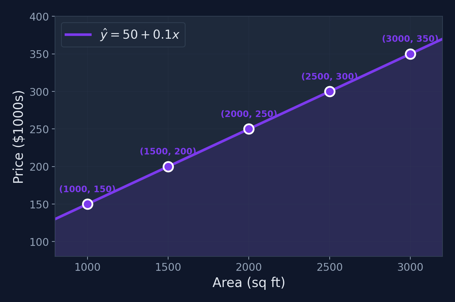
Find \(\hat{y} = w_0 + w_1 x\) that best fits this data.
Computing the Slope \(w_1\)
$$w_1 = \frac{\sum_{i=1}^{m}(x_i - \bar{x})(y_i - \bar{y})}{\sum_{i=1}^{m}(x_i - \bar{x})^2}$$
Step 1: Compute means
\(\bar{x} = \frac{1000+1500+2000+2500+3000}{5} = 2000\)
\(\bar{y} = \frac{150+200+250+300+350}{5} = 250\)
Step 2: Compute sums
Numerator: \(250{,}000\)
Denominator: \(2{,}500{,}000\)
\(w_1 = \frac{250{,}000}{2{,}500{,}000} = \mathbf{0.1}\)
Intercept & Final Model
$$w_0 = \bar{y} - w_1 \bar{x} = 250 - 0.1 \times 2000 = \mathbf{50}$$
Final Model: \(\hat{y} = 50 + 0.1x\)
Interpretation
- Base price: $50,000 (the intercept)
- Each additional sq ft adds $100 to the price (the slope)
Making Predictions
Using our model \(\hat{y} = 50 + 0.1x\):
| Area \(x\) | Computation | Predicted Price \(\hat{y}\) |
|---|---|---|
| 1,200 sq ft | \(50 + 0.1(1200)\) | $170K |
| 1,800 sq ft | \(50 + 0.1(1800)\) | $230K |
| 2,200 sq ft | \(50 + 0.1(2200)\) | $270K |
| 3,500 sq ft | \(50 + 0.1(3500)\) | $400K |
Key
The model can predict for any area value — even ones not in the training data.
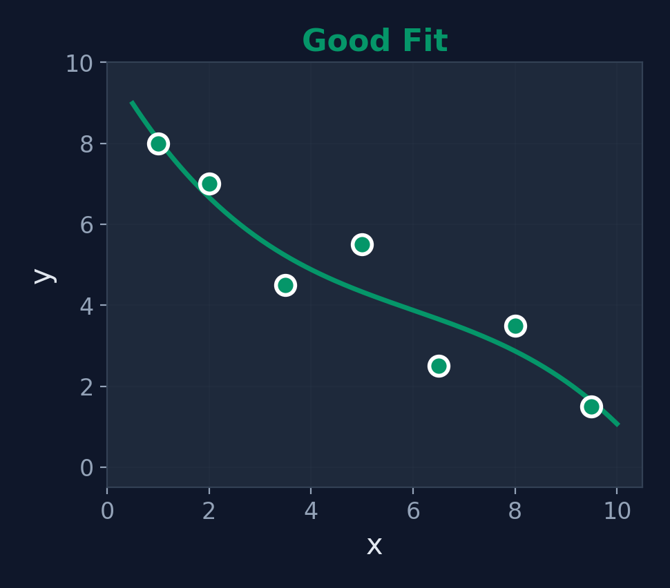
Visualization
What Does "Error" Mean?
Residuals
The vertical dashed lines are the residuals (errors): \(e_i = \hat{y}_i - y_i\). Each one measures how far off our prediction is. The "best" line minimizes these gaps overall.
Why Squared Errors?
Why not just sum the errors \(\sum(e_i)\)?
Positive and negative errors cancel out! A line through the middle of a scattered cloud could have total error = 0 despite being terrible.
Sum of errors
\(\sum e_i\)
Cancels out — useless
Absolute errors
\(\sum |e_i|\)
Works, but not differentiable at 0
Squared errors
\(\sum e_i^2\)
Always positive, differentiable, penalizes big errors more
Why "differentiable" matters
We need to take the derivative of the cost function to do gradient descent. Squared errors give us smooth derivatives — crucial for optimization.
Cost Function: Mean Squared Error
How do we measure "best fit"?
By minimizing the average squared distance between predictions and actual values.
$$J(w_0, w_1) = \frac{1}{2m}\sum_{i=1}^{m}(\hat{y}_i - y_i)^2$$
For our example
\(J = \frac{1}{10}[(150-150)^2 + (200-200)^2 + \ldots] = 0\). Perfect fit!
Next question
How do we efficiently minimize \(J\) when data isn't perfectly linear? Enter: Gradient Descent
Gradient Descent
What is Gradient Descent?
Definition
An iterative optimization algorithm that finds the minimum of a function by repeatedly taking steps proportional to the negative of the gradient.
$$w := w - \alpha \frac{\partial J}{\partial w}$$
Where \(\alpha\) is the learning rate (step size)
Intuition
Imagine standing on a foggy hill. You can only feel the slope under your feet. The gradient tells you which direction is steepest — walk the opposite way to go downhill.
Where it's used
Linear regression, logistic regression, neural networks, SVMs, transformers — virtually every ML model is trained with some form of gradient descent.
Why Do We Need Gradient Descent?
Can't we just use a formula?
For simple linear regression with 1 feature, yes — we used the closed-form formula to get \(w_1 = 0.1\). But what about...
Formula fails when...
- You have 100+ features (matrix inversion is \(O(n^3)\))
- The model is non-linear (neural networks)
- Dataset is too large for memory
GD works for...
- Any differentiable function
- Any number of parameters
- Any dataset size (mini-batches)
- Linear models and neural networks
Gradient descent is the universal optimizer — it's how we train everything from logistic regression to GPT-4.
The Calculus You Need: 3 Rules
What is a derivative?
The derivative \(\frac{df}{dx}\) tells you the slope (rate of change) of \(f\) at any point. Positive slope = function is increasing. Negative slope = decreasing.
| Rule | Formula | Example |
|---|---|---|
| Power Rule | \(\frac{d}{dx}[x^n] = nx^{n-1}\) | \(\frac{d}{dx}[x^2] = 2x\) |
| Constant Rule | \(\frac{d}{dx}[cf(x)] = c \cdot f'(x)\) | \(\frac{d}{dx}[3x^2] = 6x\) |
| Chain Rule | \(\frac{d}{dx}[f(g(x))] = f'(g(x)) \cdot g'(x)\) | \(\frac{d}{dx}[(2x+1)^2] = 2(2x+1) \cdot 2\) |
That's it!
With these 3 rules, you can derive every gradient in this lecture. Let's try it on MSE.
Intuition: Rolling Downhill
Imagine
You're standing on a hillside in dense fog. You can only feel the slope under your feet.
Strategy: Always step in the steepest downhill direction. Eventually, you reach the valley (minimum).
Why the Negative Gradient?
If gradient is negative
Subtracting a negative number = adding → we move right (toward the minimum)
If gradient is positive
Subtracting a positive number = decreasing → we move left (toward the minimum)
Either way, the negative gradient always points toward the minimum!
Use Cases for Gradient Descent
Training Neural Networks
Optimize millions of weights via backpropagation
Linear/Logistic Regression
Find optimal parameters for prediction models
Image Recognition
Train CNNs for object detection and classification
Natural Language Processing
Train transformers for language understanding
The Gradient Descent Algorithm
1. Initialize weights w randomly
2. Repeat until convergence:
   a. Compute gradient: g = dJ/dw
   b. Update weights:  w = w - α × g
3. Return w
Key insight
The gradient \(\frac{\partial J}{\partial w}\) tells us the direction of steepest ascent. We go in the opposite direction (hence the minus sign).
Deriving the MSE Gradient — Setup
Our cost function (MSE)
$$J(w_0, w_1) = \frac{1}{2m}\sum_{i=1}^{m}(\hat{y}_i - y_i)^2$$
Substitute the model
Since \(\hat{y}_i = w_0 + w_1 x_i\), we can write:
$$J(w_0, w_1) = \frac{1}{2m}\sum_{i=1}^{m}(w_0 + w_1 x_i - y_i)^2$$
We need two partial derivatives
\(\frac{\partial J}{\partial w_1}\) — how does the cost change when we adjust the slope?
\(\frac{\partial J}{\partial w_0}\) — how does the cost change when we adjust the intercept?
Deriving \(\frac{\partial J}{\partial w_1}\) — Step by Step
Step 1: Apply the derivative to the sum
$$\frac{\partial J}{\partial w_1} = \frac{1}{2m}\sum_{i=1}^{m} \frac{\partial}{\partial w_1}\left[(w_0 + w_1 x_i - y_i)^2\right]$$
Step 2: Chain rule — derivative of \((\text{something})^2\)
$$= \frac{1}{2m}\sum_{i=1}^{m} 2(w_0 + w_1 x_i - y_i) \cdot \frac{\partial}{\partial w_1}(w_0 + w_1 x_i - y_i)$$
The inner derivative w.r.t. \(w_1\): \(\frac{\partial}{\partial w_1}(w_0 + w_1 x_i - y_i) = x_i\)
Step 3: Simplify — the 2 and \(\frac{1}{2}\) cancel!
$$= \frac{1}{m}\sum_{i=1}^{m}(w_0 + w_1 x_i - y_i) \cdot x_i$$
$$\boxed{\frac{\partial J}{\partial w_1} = \frac{1}{m}\sum_{i=1}^{m}(\hat{y}_i - y_i) \cdot x_i}$$
Deriving \(\frac{\partial J}{\partial w_0}\) — Step by Step
Same process, but the inner derivative changes
$$\frac{\partial J}{\partial w_0} = \frac{1}{2m}\sum_{i=1}^{m} 2(w_0 + w_1 x_i - y_i) \cdot \frac{\partial}{\partial w_0}(w_0 + w_1 x_i - y_i)$$
Key difference
\(\frac{\partial}{\partial w_0}(w_0 + w_1 x_i - y_i) = \mathbf{1}\)
Compare: for \(w_1\) it was \(x_i\)
Result
$$\frac{\partial J}{\partial w_0} = \frac{1}{m}\sum_{i=1}^{m}(\hat{y}_i - y_i)$$
No \(x_i\) — just the average error!
Intuition: \(\frac{\partial J}{\partial w_0}\) is the average prediction error. \(\frac{\partial J}{\partial w_1}\) is the error weighted by the input — larger inputs contribute more.
The Complete Update Rules
Gradient Descent for Linear Regression
$$w_1 := w_1 - \alpha \cdot \frac{1}{m}\sum_{i=1}^{m}(\hat{y}_i - y_i) \cdot x_i$$
$$w_0 := w_0 - \alpha \cdot \frac{1}{m}\sum_{i=1}^{m}(\hat{y}_i - y_i)$$
What we derived
- Start from the cost function \(J\)
- Take partial derivatives using chain rule
- Get the gradients for each parameter
- Subtract them (scaled by \(\alpha\))
Two equations — that's it!
These two equations are all you need to train linear regression. Repeat until convergence.
GD for Linear Regression — Worked Example
Using our house price data (5 points)
Start: \(w_0 = 0,\; w_1 = 0,\; \alpha = 0.0000001\) (tiny LR because features are large)
Iteration 0: Compute predictions (\(\hat{y} = 0 + 0 \cdot x = 0\) for all)
Errors: \(\hat{y}_i - y_i = [0-150,\; 0-200,\; 0-250,\; 0-300,\; 0-350] = [-150, -200, -250, -300, -350]\)
\(\frac{\partial J}{\partial w_0}\)
\(= \frac{1}{5}(-150-200-250-300-350)\)
\(= \frac{-1250}{5} = \mathbf{-250}\)
\(\frac{\partial J}{\partial w_1}\)
\(= \frac{1}{5}[(-150)(1000) + (-200)(1500) + \ldots]\)
\(= \frac{-575{,}000}{5} \times 10^{-7} \approx \mathbf{-550{,}000}\)
Update
\(w_0' = 0 - 10^{-7}(-250) = 0.000025\), \(w_1' = 0 - 10^{-7}(-550000) = 0.055\). One step closer!
GD for Linear Regression — Convergence
| Iteration | \(w_0\) | \(w_1\) | \(J\) (cost) |
|---|---|---|---|
| 0 | 0.000 | 0.000 | 32,500 |
| 10 | 0.003 | 0.042 | 10,240 |
| 100 | 0.28 | 0.084 | 1,056 |
| 1,000 | 12.4 | 0.097 | 28.7 |
| 10,000 | 45.8 | 0.100 | 0.35 |
| ~50,000 | 50.0 | 0.100 | ≈ 0 |
Same answer!
GD converges to \(w_0 = 50,\; w_1 = 0.1\) — exactly the same as the closed-form formula.
But GD generalizes
Unlike the formula, GD works for any differentiable model — logistic regression, neural networks, transformers...
Worked Example: Setup
Problem
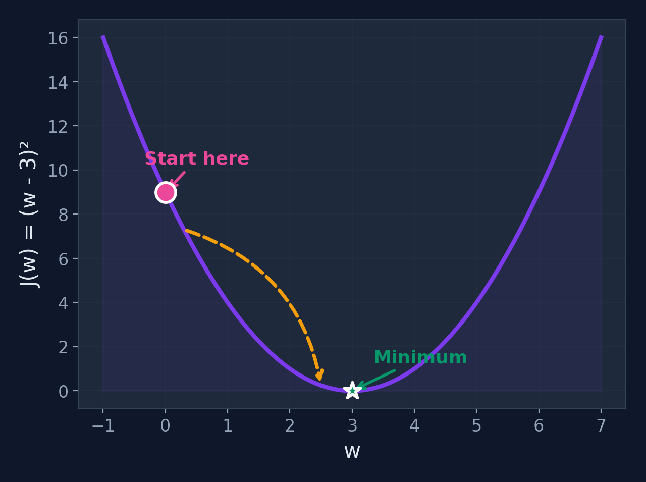
Minimize \(J(w) = (w - 3)^2\)
Settings
- Starting point: \(w_0 = 0\)
- Learning rate: \(\alpha = 0.2\)
- Gradient: \(\frac{dJ}{dw} = 2(w - 3)\)
Expected minimum
\(J(w)\) is minimized when \(w = 3\). Let's see if gradient descent finds it!
What we expect
Since \(J(w) = (w-3)^2\) is a perfect parabola with minimum at \(w=3\), GD should converge there. Starting at \(w=0\), the gradient is negative (slope points downhill to the right), so GD will move \(w\) to the right toward 3.
Step-by-Step Iterations
| Iter | \(w\) | \(\frac{dJ}{dw} = 2(w-3)\) | Update | New \(w\) |
|---|---|---|---|---|
| 0 | 0.000 | \(2(0-3) = -6.0\) | \(0 - 0.2(-6.0)\) | 1.200 |
| 1 | 1.200 | \(2(1.2-3) = -3.6\) | \(1.2 - 0.2(-3.6)\) | 1.920 |
| 2 | 1.920 | \(2(1.92-3) = -2.16\) | \(1.92 - 0.2(-2.16)\) | 2.352 |
| 3 | 2.352 | \(2(2.352-3) = -1.296\) | \(2.352 - 0.2(-1.296)\) | 2.611 |
| 4 | 2.611 | \(2(2.611-3) = -0.778\) | \(2.611 - 0.2(-0.778)\) | 2.767 |
Converging toward \(w = 3\)! Each step gets us closer to the minimum.
Gradient Descent in Action
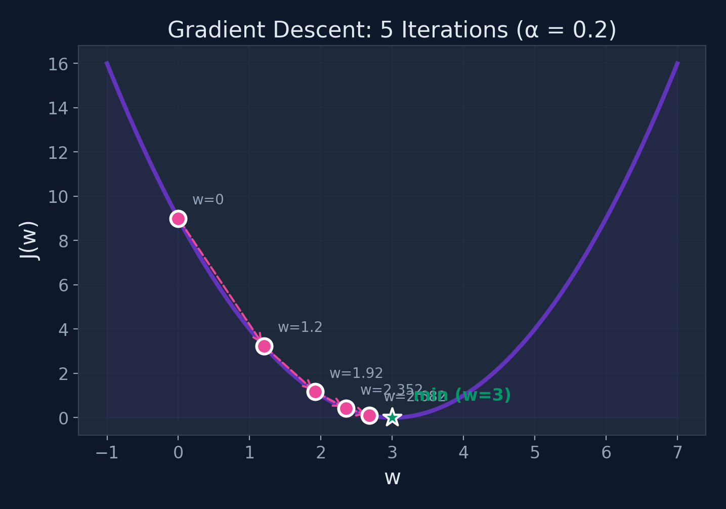
Steps get smaller as we approach the minimum — the gradient decreases!
Effect of Learning Rate \(\alpha\)
Too Small (\(\alpha = 0.01\))

Slow convergence
Just Right (\(\alpha = 0.2\))
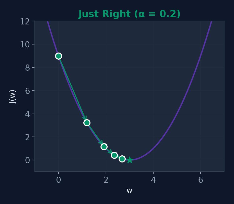
Optimal convergence
Too Large (\(\alpha = 0.9\))
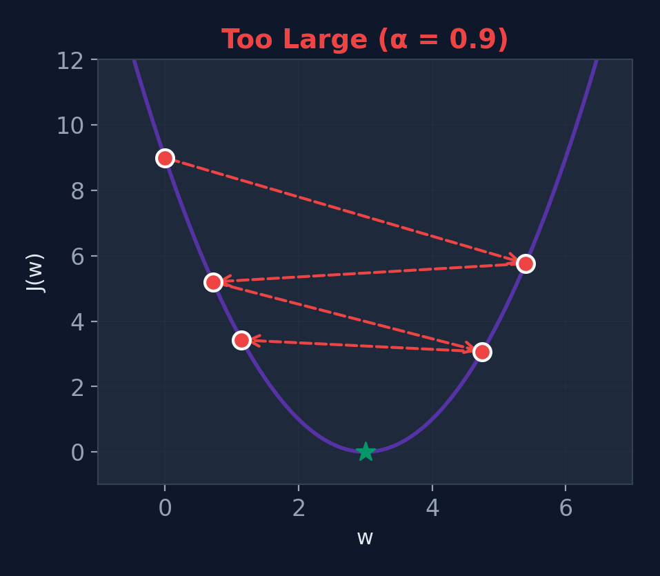
Overshoots — may diverge!
Common Pitfalls
Local Minima
Non-convex functions have multiple valleys. GD might get stuck in a shallow one instead of finding the deepest.
Saddle Points
Points where gradient = 0 but it's not a minimum. The surface curves up in one direction and down in another.
Feature Scaling
If features have very different ranges (e.g., age 0–100 vs salary 0–1M), GD zig-zags instead of going straight to the minimum.
When to Stop?
Common criteria: gradient < threshold, cost change < \(\epsilon\), or fixed number of iterations.
Good news for linear regression
MSE is convex (one valley), so GD always finds the global minimum. Neural networks? Not so lucky — but it works anyway!
Gradient Descent Variants
| Variant | Data per Step | Speed | Stability |
|---|---|---|---|
| Batch GD | All samples | Slow | Very stable |
| Stochastic GD | 1 sample | Fast | Noisy |
| Mini-batch GD | \(k\) samples | Balanced | Balanced |
In practice
Mini-batch gradient descent (batch size 32–256) is the standard in deep learning. It balances speed with stable convergence.
Logistic Regression
Why Not Linear Regression for Classification?
Problem 1
Linear regression can predict -0.2 or 1.3 — what does a negative probability mean?
Problem 2
A single outlier can shift the entire line, changing the decision boundary dramatically.
We need a function that squishes any real number into the range \((0, 1)\) → Enter: the sigmoid function
What is Logistic Regression?
Definition
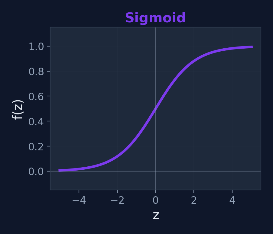
A classification algorithm that models the probability of a binary outcome using the sigmoid (logistic) function.
$$\sigma(z) = \frac{1}{1 + e^{-z}}$$
$$P(y=1|\mathbf{x}) = \sigma(\mathbf{w}^T \mathbf{x} + b)$$
Key insight
The sigmoid maps any real number to \((0, 1)\) — perfect for probabilities. Output > 0.5 → class 1, otherwise class 0.
Why "logistic"?
Named after the logistic function, coined by Pierre-François Verhulst (1845) to model population growth. Same S-curve, different application!
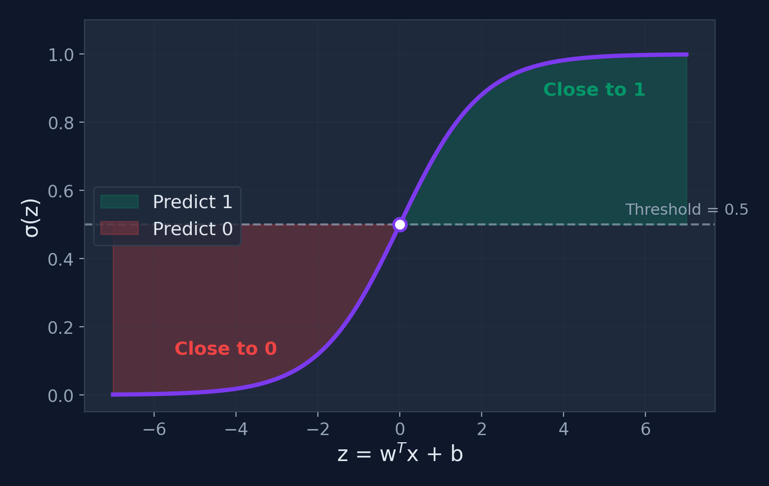
The Sigmoid Function
Sigmoid — Computing by Hand
| \(z\) | \(e^{-z}\) | \(1 + e^{-z}\) | \(\sigma(z) = \frac{1}{1+e^{-z}}\) | Interpretation |
|---|---|---|---|---|
| \(-3\) | \(e^3 = 20.09\) | \(21.09\) | 0.047 | Very likely class 0 |
| \(-1\) | \(e^1 = 2.718\) | \(3.718\) | 0.269 | Probably class 0 |
| \(0\) | \(e^0 = 1\) | \(2\) | 0.500 | Coin flip! |
| \(1\) | \(e^{-1} = 0.368\) | \(1.368\) | 0.731 | Probably class 1 |
| \(3\) | \(e^{-3} = 0.050\) | \(1.050\) | 0.953 | Very likely class 1 |
Symmetry
\(\sigma(0) = 0.5\) always. The function is symmetric around \(z = 0\).
Saturation
For \(|z| > 5\), the sigmoid is nearly 0 or 1. The neuron is "very confident."
From Probability to Decision
Linear Combination
\(z = \mathbf{w}^T\mathbf{x} + b\)
Can be any real number
Apply Sigmoid
\(p = \sigma(z)\)
Squished to (0, 1)
Apply Threshold
\(p \geq 0.5 \rightarrow\) Class 1
\(p < 0.5 \rightarrow\) Class 0
Use Cases for Logistic Regression
Email Spam Detection
Classify emails as spam or not spam
Medical Diagnosis
Predict disease presence from symptoms
Fraud Detection
Flag suspicious credit card transactions
Student Pass/Fail
Predict outcome from study hours
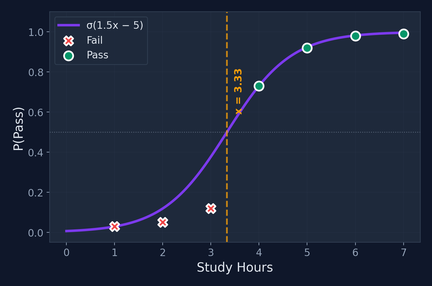
Worked Example: Setup
Problem
Predict pass/fail from study hours
| Hours \(x\) | 1 | 2 | 3 | 4 | 5 | 6 | 7 |
|---|---|---|---|---|---|---|---|
| Result | Fail | Fail | Fail | Pass | Pass | Pass | Pass |
Assume pre-trained weights
\(w_1 = 1.5\), \(b = -5.0\). Model: \(\hat{y} = \sigma(1.5x - 5.0)\), threshold = 0.5
Forward Pass Computation
| Hours \(x\) | \(z = 1.5x - 5.0\) | \(\sigma(z) = \frac{1}{1+e^{-z}}\) | Prediction |
|---|---|---|---|
| 2 | \(1.5(2)-5 = -2.0\) | \(\frac{1}{1+e^{2.0}} = 0.119\) | Fail ✗ |
| 3 | \(1.5(3)-5 = -0.5\) | \(\frac{1}{1+e^{0.5}} = 0.378\) | Fail ✗ |
| 4 | \(1.5(4)-5 = 1.0\) | \(\frac{1}{1+e^{-1.0}} = 0.731\) | Pass ✓ |
| 5 | \(1.5(5)-5 = 2.5\) | \(\frac{1}{1+e^{-2.5}} = 0.924\) | Pass ✓ |
All predictions match! The sigmoid converts the linear score into a probability.
Loss: Binary Cross-Entropy
$$J = -\frac{1}{m}\sum_{i=1}^{m}\left[y_i \log(\hat{y}_i) + (1-y_i)\log(1-\hat{y}_i)\right]$$
Why not MSE?
MSE with sigmoid creates a non-convex loss surface with many local minima. Cross-entropy is convex — gradient descent always finds the global minimum.
Intuition
- If true label = 1 and we predict 0.01 → huge penalty
- If true label = 1 and we predict 0.99 → tiny penalty
- Penalizes confident wrong predictions heavily
Decision Boundary
Training Logistic Regression
Gradient of cross-entropy
$$\frac{\partial J}{\partial w_j} = \frac{1}{m}\sum_{i=1}^{m}(\hat{y}_i - y_i)x_j^{(i)}$$
Surprise! This looks identical to the linear regression gradient — but \(\hat{y}\) uses the sigmoid.
Training recipe
- Compute predictions: \(\hat{y} = \sigma(\mathbf{w}^T\mathbf{x} + b)\)
- Compute loss: \(J\) (cross-entropy)
- Compute gradients: \(\frac{\partial J}{\partial w}\)
- Update weights: \(w := w - \alpha \nabla J\)
- Repeat until convergence
Linear vs Logistic Regression
| Feature | Linear Regression | Logistic Regression |
|---|---|---|
| Output | Continuous value | Probability (0–1) |
| Activation | None (identity) | Sigmoid |
| Loss Function | Mean Squared Error | Binary Cross-Entropy |
| Use Case | Regression (predict amount) | Classification (predict class) |
| Decision | No threshold | Threshold at 0.5 |
Key insight
Logistic regression is essentially linear regression + sigmoid. This idea of "linear combination + activation" is the foundation of neural networks!
Regularization
What is Regularization?
Definition
A technique that adds a penalty term to the loss function to prevent overfitting by discouraging overly complex models.
$$J_{\text{reg}} = J_{\text{original}} + \lambda \cdot R(\mathbf{w})$$
Where \(\lambda\) controls regularization strength
Think of it as...
Regularization is like a teacher telling a student: "I don't just want the right answer — I want a simple explanation." Simpler models generalize better.
Without regularization
Models may memorize training data instead of learning general patterns — performing perfectly on training data but failing on new data.
The \(\lambda\) dial
\(\lambda = 0\): no penalty (may overfit). \(\lambda \to \infty\): all weights → 0 (underfits). Cross-validation finds the sweet spot.
The Overfitting Analogy
The Memorizer
Memorizes every answer from past exams word-for-word
The Understander
Learns the underlying concepts and problem-solving strategies
Regularization forces the model to "understand" rather than "memorize" — slightly worse on training data, much better on new data.
Underfitting vs. Just Right vs. Overfitting
Underfitting
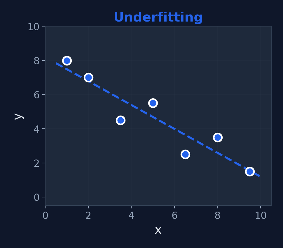
High Bias — too simple
Just Right
Good Balance
Overfitting
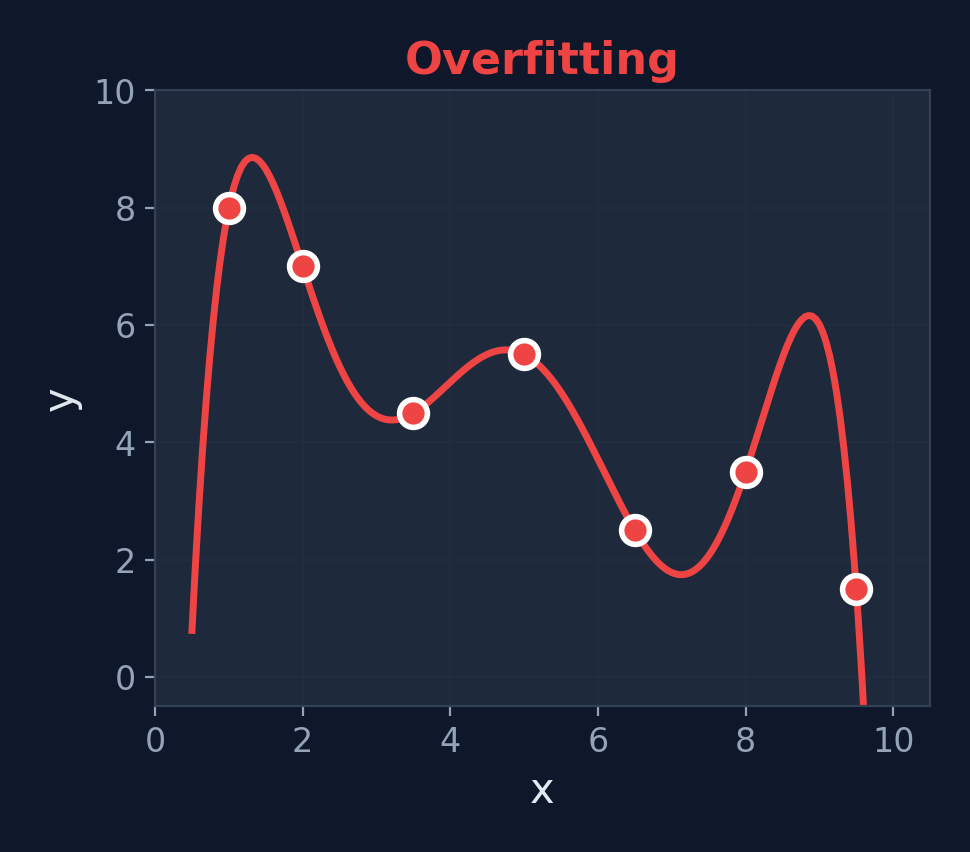
High Variance — too complex
Types of Regularization
L1 Regularization (Lasso)
$$J_{L1} = J + \lambda \sum_{i} |w_i|$$
Encourages sparsity — some weights become exactly 0, effectively performing feature selection.
L2 Regularization (Ridge)
$$J_{L2} = J + \lambda \sum_{i} w_i^2$$
Shrinks all weights toward 0 but never exactly 0. Smoother, more stable solutions.
When to use L1
You suspect many features are irrelevant and want the model to automatically ignore them. L1 acts as a built-in feature selector.
When to use L2
All features matter but you want to prevent any single weight from dominating. L2 keeps everything small and balanced — the default choice.
Beyond L1 & L2: More Techniques
Elastic Net (L1 + L2)
$$J_{EN} = J + \lambda_1 \sum|w_i| + \lambda_2 \sum w_i^2$$
Combines the best of both: feature selection and weight shrinkage. Used in scikit-learn's ElasticNet.
Dropout (Neural Networks)
Randomly "turn off" neurons during training (e.g., 50% chance). Forces the network to not rely on any single neuron.
Like studying with random pages removed — you learn the core concepts, not surface patterns.
Preview
We'll explore dropout in detail when we cover deep network training. For now, remember: regularization = adding constraints to prevent overfitting.
Use Cases for Regularization
Feature Selection (L1)
Automatically remove irrelevant features by zeroing their weights
Neural Network Training
Prevent deep networks from memorizing training data
Reducing Complexity
Keep models simple and interpretable
Improving Generalization
Models perform better on unseen test data
Worked Example: L2 Regularization
Applying L2 penalty to our linear regression
Original model: \(w_0 = 50\) (bias), \(w_1 = 0.1\) (weight), and \(\lambda = 0.01\)
Without regularization
\(J = 0\) (perfect fit)
With L2 regularization
\(J_{\text{reg}} = 0 + 0.01 \times (0.1^2) = 0 + 0.01 \times 0.01 = \mathbf{0.0001}\)
Updated gradient
\(\frac{\partial J_{\text{reg}}}{\partial w_j} = \frac{\partial J}{\partial w_j} + 2\lambda w_j\) — only feature weights; bias \(w_0\) is not penalized. The penalty pushes large weights smaller during training.
Effect of \(\lambda\)
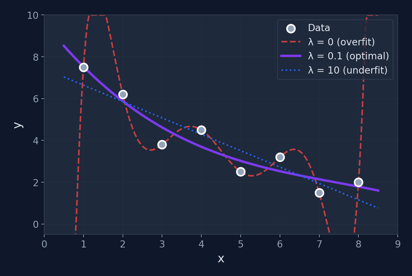
Regularization Summary
Key Takeaways
- Regularization controls model complexity via a penalty term
- L1 (Lasso): Feature selection (sparse weights)
- L2 (Ridge): Weight shrinkage (smooth models)
- \(\lambda\) balances fit quality vs. complexity
- Elastic Net: Combines L1 + L2 (best of both)
What's Next?
We now have the classical building blocks:
- Regression (linear & logistic)
- Optimization (gradient descent)
- Regularization (preventing overfitting)
Let's look at the history that led from these ideas to neural networks...
Cheat Sheet
| Method | Penalty | Effect | Best for |
|---|---|---|---|
| L1 | \(\lambda\sum|w_i|\) | Zeros out weights | Feature selection |
| L2 | \(\lambda\sum w_i^2\) | Shrinks weights | Preventing large weights |
| Elastic Net | L1 + L2 | Both | Correlated features |
| Dropout | Random neuron removal | Ensemble effect | Neural networks |
A Brief History of Neural Networks
From the 1940s to Today
The Early Years (1943–1969)
McCulloch & Pitts — First mathematical model of an artificial neuron. Showed neurons could compute logical functions.
Frank Rosenblatt's Perceptron — First trainable neural network, implemented in hardware. Could learn to classify simple patterns.
Minsky & Papert — Published "Perceptrons", proving single-layer networks cannot solve XOR. Revealed fundamental limitations.
First AI Winter (1970s)
Funding and interest dried up. Neural network research was largely abandoned for over a decade.
The Resurgence (1986–2006)
Rumelhart, Hinton & Williams — Popularized backpropagation, enabling training of multi-layer networks. The key breakthrough.
Yann LeCun — Applied CNNs to handwritten digit recognition (MNIST). First practical deep learning success.
Hochreiter & Schmidhuber — Invented LSTM for sequential data, solving the vanishing gradient problem.
Geoffrey Hinton — Deep Belief Networks. The term "Deep Learning" enters mainstream AI vocabulary.
Why backpropagation mattered
Before 1986, there was no efficient way to train multi-layer networks. Backpropagation gave us a systematic method to compute gradients for every weight — not just the output layer, but all hidden layers too. This was the missing piece.
The Deep Learning Era (2012–Present)
AlexNet wins ImageNet by a huge margin. 8 layers, GPU training. The "Big Bang" of modern deep learning.
GANs (Goodfellow) — Generative Adversarial Networks can create realistic images from noise.
"Attention Is All You Need" — The Transformer architecture revolutionizes NLP and later all of AI.
ChatGPT & LLMs — Large language models reach mainstream. AI becomes a daily tool for millions.
Why Neural Networks Work Now
Big Data
Internet, smartphones, and sensors generate massive datasets. Deep networks need lots of data to learn effectively.
Compute Power
GPUs, TPUs, and cloud computing make training billion-parameter models feasible. 10,000x faster than 2000s hardware.
Better Algorithms
ReLU, batch normalization, dropout, residual connections, Adam optimizer — all invented in the 2010s.
From Classical ML to Neural Networks
Everything connects
A neural network is built from the same building blocks we've been studying — weighted sums, activation functions, and gradient-based optimization.
Think-Pair-Share
Discussion Question
Why did neural networks fail in the 1970s but succeed in the 2010s?
What changed in terms of data, compute, and algorithms?
Hint: Data
How much data existed in the 1970s vs. the age of the internet?
Hint: Compute
What hardware breakthrough made matrix multiplication 100× faster?
Hint: Algorithms
What training method was missing before 1986?
Click to reveal answer
1970s: Limited data, no GPUs, only single-layer networks (couldn't solve XOR). 2010s: Internet-scale data, GPU parallelism (NVIDIA CUDA), and breakthroughs like backpropagation, ReLU, and batch normalization made deep networks trainable.
The Simple Neuron
The Perceptron
What is an Artificial Neuron?
Definition
A computational unit that takes weighted inputs, sums them, adds a bias, and applies an activation function.
$$z = \sum_{i=1}^{n} w_i x_i + b, \quad a = f(z)$$
Biological vs. Artificial
Mapping
| Dendrites | → Inputs \(x_1, x_2, \ldots\) |
| Synaptic strength | → Weights \(w_1, w_2, \ldots\) |
| Soma (cell body) | → Summation \(\Sigma\) |
| Axon hillock | → Activation function \(f\) |
| Axon | → Output \(\hat{y}\) |
Important caveat
Real neurons are vastly more complex — they use timing, chemical signals, and recurrent connections. The artificial neuron is a very rough approximation.
Common Activation Functions
Sigmoid
\(f(z) = \frac{1}{1+e^{-z}}\)
Range: (0, 1)
ReLU
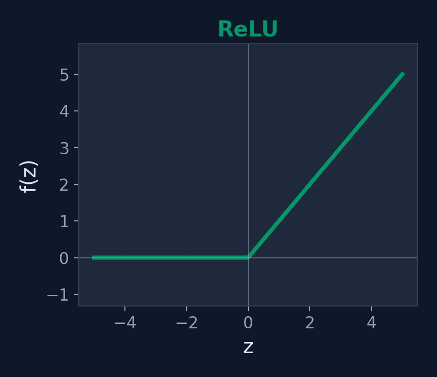
\(f(z) = \max(0, z)\)
Range: [0, ∞)
Tanh
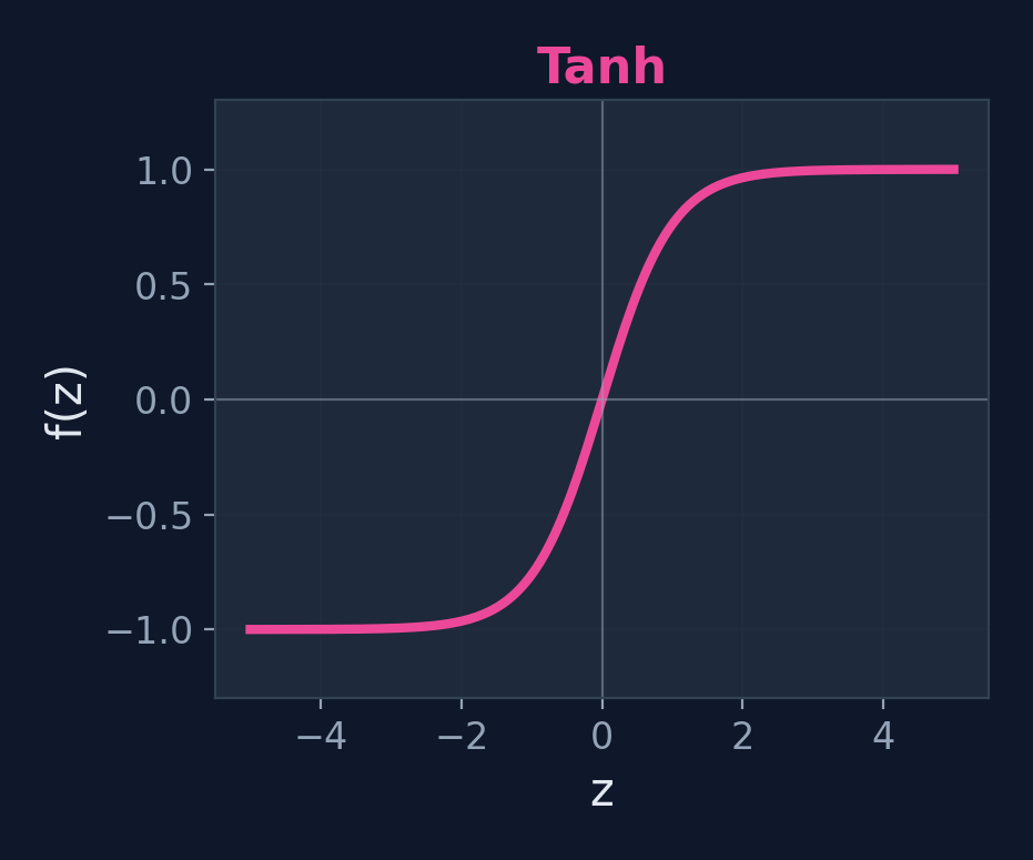
\(f(z) = \tanh(z)\)
Range: (-1, 1)
Modern default: ReLU
Fast to compute, avoids vanishing gradient problem, works well in practice.
What Can a Single Neuron Do?
Key Insight
A single neuron with sigmoid activation is logistic regression! Same weighted sum + same activation function.
Capabilities
- Binary classification
- Logic gates: AND, OR, NOT
- Any linearly separable problem
Limitations
- Cannot solve XOR
- Cannot learn non-linear boundaries
- Only one decision boundary (a line/plane)
Worked Example: AND Gate
Neuron
\(w_1 = 1,\; w_2 = 1,\; b = -1.5\), step activation \(f(z) = \begin{cases}1 & z \geq 0\\0 & z < 0\end{cases}\)
| \(x_1\) | \(x_2\) | \(z = x_1 + x_2 - 1.5\) | \(f(z)\) | AND | Match? |
|---|---|---|---|---|---|
| 0 | 0 | \(0 + 0 - 1.5 = -1.5\) | 0 | 0 | ✓ |
| 0 | 1 | \(0 + 1 - 1.5 = -0.5\) | 0 | 0 | ✓ |
| 1 | 0 | \(1 + 0 - 1.5 = -0.5\) | 0 | 0 | ✓ |
| 1 | 1 | \(1 + 1 - 1.5 = 0.5\) | 1 | 1 | ✓ |
The perceptron correctly computes AND! A single neuron can learn any linearly separable function.
OR Gate — Change the Bias!
Neuron
\(w_1 = 1,\; w_2 = 1,\; b = -0.5\), same step activation
| \(x_1\) | \(x_2\) | \(z = x_1 + x_2 - 0.5\) | \(f(z)\) | OR | Match? |
|---|---|---|---|---|---|
| 0 | 0 | \(0 + 0 - 0.5 = -0.5\) | 0 | 0 | ✓ |
| 0 | 1 | \(0 + 1 - 0.5 = 0.5\) | 1 | 1 | ✓ |
| 1 | 0 | \(1 + 0 - 0.5 = 0.5\) | 1 | 1 | ✓ |
| 1 | 1 | \(1 + 1 - 0.5 = 1.5\) | 1 | 1 | ✓ |
Just by changing the bias from \(-1.5\) to \(-0.5\), the neuron switches from AND to OR!
NOT Gate — Single Input
Neuron
\(w_1 = -1,\; b = 0.5\), step activation. Only one input.
| \(x\) | \(z = -x + 0.5\) | \(f(z)\) | NOT \(x\) | Match? |
|---|---|---|---|---|
| 0 | \(-0 + 0.5 = 0.5\) | 1 | 1 | ✓ |
| 1 | \(-1 + 0.5 = -0.5\) | 0 | 0 | ✓ |
Key insight
With AND, OR, and NOT, neurons can compute any Boolean function... if we stack them in layers.
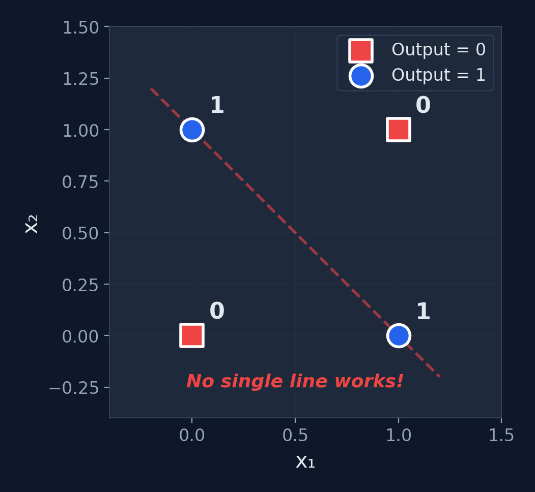
The XOR Problem
Can a single neuron compute XOR?
| \(x_1\) | \(x_2\) | XOR |
|---|---|---|
| 0 | 0 | 0 |
| 0 | 1 | 1 |
| 1 | 0 | 1 |
| 1 | 1 | 0 |
No! XOR is not linearly separable. No single straight line can separate the 1s from the 0s.
AND Gate Neuron — Traced
Step-by-step for input (1, 1)
- \(z = w_1 x_1 + w_2 x_2 + b\)
- \(z = 1(1) + 1(1) + (-1.5)\)
- \(z = 2 - 1.5 = 0.5\)
- \(f(0.5) = 1\) (since \(0.5 \geq 0\))
Output: 1 ✓ Correct!
We Need More Power
The Limitation
A single neuron can only learn linearly separable patterns. It draws one straight line through feature space.
The Solution
Stack multiple neurons in layers. Each neuron learns a different feature. Together, they can solve XOR and any non-linear problem!
Enter: The Multilayer Perceptron (MLP)
Mathematical proof
Minsky & Papert (1969) formally proved no single perceptron can solve XOR. This wasn't opinion — it was a theorem. The search for multilayer networks was the direct response.
The key insight
One hidden neuron can learn one decision boundary. Two hidden neurons = two boundaries. Combined, they carve out any region in feature space.
Multilayer Perceptron
Hidden Layers
What is an MLP?
Definition
A feedforward neural network with one or more hidden layers between the input and output layers. Each layer is fully connected to the next.
Structure
Input Layer → Hidden Layer(s) → Output Layer
- Each connection has a weight
- Each neuron has a bias and activation function
- Information flows forward only (no loops)
Universal Approximation Theorem
An MLP with just one hidden layer (enough neurons) can approximate any continuous function. This was proven by Cybenko in 1989.
Terminology
Feedforward = data flows one direction. Dense layer = fully connected layer. Hidden = not directly observed (neither input nor output).
What Hidden Layers Actually Learn
Layer 1: Edges
Detects simple patterns — lines, curves, light/dark transitions
Layer 2: Parts
Combines edges into shapes — eyes, noses, wheels, letters
Layer 3: Objects
Combines parts into concepts — faces, cars, words
Key insight
Each layer builds more abstract representations from the layer before. The network automatically learns what features matter — no manual feature engineering needed.
MLP Architecture
Reading the diagram
Each circle = a neuron. Each line = a weight. Blue = inputs, purple = hidden neurons, green = output.
Parameter count
Weights: \(2 \times 3 + 3 \times 1 = 9\). Biases: \(3 + 1 = 4\). Total: 13 parameters.
Use Cases for MLP
XOR & Non-Linear Classification
Solve problems that single neurons cannot
Handwritten Digit Recognition
MNIST dataset — the "Hello World" of deep learning
Function Approximation
Universal approximation theorem: can approximate any continuous function
Tabular Data Prediction
Structured data with complex feature interactions
Solving XOR with an MLP
Network
2 inputs, 2 hidden neurons (step activation), 1 output
Hidden neuron \(h_1\) (OR-like)
\(w_{11}=1,\; w_{12}=1,\; b_1=-0.5\)
\(h_1 = f(x_1 + x_2 - 0.5)\)
Hidden neuron \(h_2\) (AND)
\(w_{21}=1,\; w_{22}=1,\; b_2=-1.5\)
\(h_2 = f(x_1 + x_2 - 1.5)\)
Output neuron
\(v_1 = 1,\; v_2 = -2,\; b_o = -0.5\). \(\hat{y} = f(h_1 - 2h_2 - 0.5)\) — computes "\(h_1\) AND NOT \(h_2\)"
XOR — Full Computation
| \(x_1\) | \(x_2\) | \(h_1\) = f(\(x_1+x_2-0.5\)) | \(h_2\) = f(\(x_1+x_2-1.5\)) | \(\hat{y}\) = f(\(h_1-2h_2-0.5\)) | XOR | |
|---|---|---|---|---|---|---|
| 0 | 0 | f(-0.5) = 0 | f(-1.5) = 0 | f(-0.5) = 0 | 0 | ✓ |
| 0 | 1 | f(0.5) = 1 | f(-0.5) = 0 | f(0.5) = 1 | 1 | ✓ |
| 1 | 0 | f(0.5) = 1 | f(-0.5) = 0 | f(0.5) = 1 | 1 | ✓ |
| 1 | 1 | f(1.5) = 1 | f(0.5) = 1 | f(-1.5) = 0 | 0 | ✓ |
XOR Solved! The hidden layer creates intermediate features that make the problem linearly separable.
Backpropagation: The Key Idea
The Problem
We know the output is wrong, but how do we know which hidden weights to blame? The hidden neurons don't have direct targets — only the output does.
Factory Analogy
Imagine a factory assembly line with 3 stations. The final product is defective. You trace backward:
- Station 3 (output): added the wrong label → fix station 3
- Station 2 (hidden): provided a bent component → fix station 2
- Station 1 (hidden): cut the material too short → fix station 1
Backpropagation does exactly this — it traces the error backward through each layer.
The math tool that makes this possible: the chain rule from calculus.
Training MLPs: Backpropagation
Forward Pass
- Feed input through network
- Compute each layer's output
- Get final prediction \(\hat{y}\)
- Compute loss \(J\)
Backward Pass
- Compute output error
- Propagate error backward
- Compute gradients via chain rule
- Update all weights
Chain Rule
$$\frac{\partial J}{\partial w^{[l]}} = \frac{\partial J}{\partial a^{[L]}} \cdot \frac{\partial a^{[L]}}{\partial z^{[L]}} \cdot \ldots \cdot \frac{\partial z^{[l]}}{\partial w^{[l]}}$$
Backpropagation = the chain rule applied systematically across layers
Backprop Example: Forward Pass
Tiny network: 1 input → 1 hidden (sigmoid) → 1 output (sigmoid)
Input: \(x = 1\), Target: \(y = 1\), Learning rate: \(\alpha = 0.5\)
Weights: \(w_1 = 0.5,\; b_1 = 0.2\) (hidden) | \(w_2 = 0.8,\; b_2 = 0.1\) (output)
Hidden layer
\(z_1 = w_1 x + b_1 = 0.5(1) + 0.2 = 0.7\)
\(h = \sigma(0.7) = \frac{1}{1+e^{-0.7}} = \mathbf{0.668}\)
Output layer
\(z_2 = w_2 h + b_2 = 0.8(0.668) + 0.1 = 0.634\)
\(\hat{y} = \sigma(0.634) = \frac{1}{1+e^{-0.634}} = \mathbf{0.653}\)
Loss (MSE)
\(L = \frac{1}{2}(\hat{y} - y)^2 = \frac{1}{2}(0.653 - 1)^2 = \frac{1}{2}(0.121) = \mathbf{0.0603}\). We want to reduce this!
Backprop Example: Backward Pass
Output layer gradient (\(\frac{\partial L}{\partial w_2}\))
\(\frac{\partial L}{\partial \hat{y}} = \hat{y} - y = 0.653 - 1 = -0.347\)
\(\frac{\partial \hat{y}}{\partial z_2} = \hat{y}(1-\hat{y}) = 0.653 \times 0.347 = 0.2266\) (sigmoid derivative)
\(\frac{\partial z_2}{\partial w_2} = h = 0.668\)
Chain rule: \(\frac{\partial L}{\partial w_2} = (-0.347)(0.2266)(0.668) = \mathbf{-0.0525}\)
Hidden layer gradient (\(\frac{\partial L}{\partial w_1}\))
Continue the chain through \(w_2\): \(\frac{\partial z_2}{\partial h} = w_2 = 0.8\), \(\frac{\partial h}{\partial z_1} = h(1-h) = 0.668 \times 0.332 = 0.2218\), \(\frac{\partial z_1}{\partial w_1} = x = 1\)
Chain rule: \(\frac{\partial L}{\partial w_1} = (-0.347)(0.2266)(0.8)(0.2218)(1) = \mathbf{-0.01394}\)
Backprop Example: Update & Verify
Update weights (\(\alpha = 0.5\))
\(w_2' = 0.8 - 0.5(-0.0525) = \mathbf{0.826}\)
\(w_1' = 0.5 - 0.5(-0.01394) = \mathbf{0.507}\)
Verify: new forward pass
\(z_1' = 0.507(1) + 0.2 = 0.707\)
\(h' = \sigma(0.707) = 0.670\)
\(z_2' = 0.826(0.670) + 0.1 = 0.653\)
\(\hat{y}' = \sigma(0.653) = \mathbf{0.658}\)
One step of backprop reduced the loss! Repeat this thousands of times and the network learns.
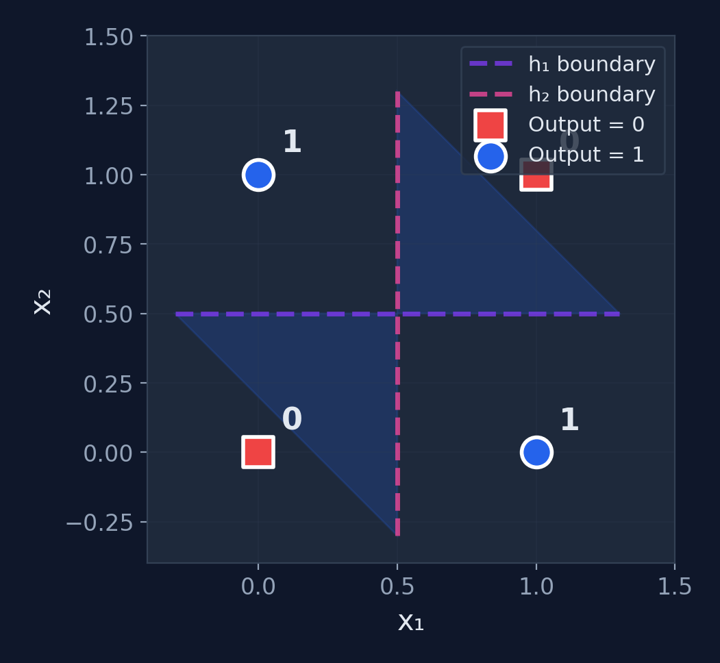
How the MLP Solves XOR
What happened?
- \(h_1\) draws one boundary line
- \(h_2\) draws another boundary line
- The output combines them: the region between the lines is class 1
- Two linear boundaries → one non-linear decision region
The power of hidden layers
They transform the input space into a representation where the problem becomes linearly separable.
Fully Connected Neural Networks
Going Deep
What is a Fully Connected Neural Network?
Definition
A deep neural network where every neuron in one layer is connected to every neuron in the next layer. Also called a Dense Network or Deep Feedforward Network.
MLP vs FCNN
An MLP with 2+ hidden layers = a Fully Connected Neural Network. "Deep" means multiple hidden layers.
Key property
More layers = more abstraction. Early layers learn simple features, deeper layers learn complex combinations.
Why "deep"?
A network with 2+ hidden layers is called "deep." More depth = more capacity to learn complex patterns. Most modern networks have 10–100+ layers.
Scale comparison
Our XOR solver: 2 layers, 13 params. MNIST digit recognizer: 2 layers, 109K params. GPT-4: ~120 layers, 1.8T params.
FCNN Architecture
Parameters: \((3 \times 4 + 4) + (4 \times 4 + 4) + (4 \times 2 + 2) = 16 + 20 + 10 = \mathbf{46}\) total
How Many Operations? Thinking About Scale
Every parameter = 1 multiply + 1 add
A forward pass through a network requires one multiplication per weight and one addition per bias. The total cost scales with parameter count.
Why GPUs matter
A CPU does operations one-by-one. A GPU does thousands in parallel. Training GPT-4 on a single CPU would take ~300 years. On 25,000 GPUs: ~3 months.
Use Cases for FCNNs
Image Classification
Flatten pixels into a vector and classify (before CNNs took over)
Natural Language Processing
Process word embeddings for sentiment analysis and text classification
Tabular / Structured Data
FCNNs remain the go-to for structured feature data (customer churn, fraud)
Reinforcement Learning
Policy and value networks in game-playing agents (DQN)
Worked Example: Forward Pass (Layer 1)
FCNN
2 inputs → 2 hidden (ReLU) → 1 output (sigmoid). Input: \(\mathbf{x} = [0.5,\; 0.8]\)
Layer 1 weights & bias
$$W^{[1]} = \begin{bmatrix} 0.2 & 0.4 \\ 0.6 & 0.3 \end{bmatrix}, \quad b^{[1]} = \begin{bmatrix} 0.1 \\ 0.2 \end{bmatrix}$$
Compute \(z^{[1]} = W^{[1]}\mathbf{x} + b^{[1]}\)
\(z_1^{[1]} = 0.2(0.5) + 0.4(0.8) + 0.1 = \mathbf{0.52}\)
\(z_2^{[1]} = 0.6(0.5) + 0.3(0.8) + 0.2 = \mathbf{0.74}\)
\(a^{[1]} = \text{ReLU}(z^{[1]}) = [\max(0, 0.52),\; \max(0, 0.74)] = \mathbf{[0.52,\; 0.74]}\)
Worked Example: Forward Pass (Output)
Layer 2 (output) weights & bias
$$W^{[2]} = \begin{bmatrix} 0.5 & 0.7 \end{bmatrix}, \quad b^{[2]} = 0.1$$
Compute output
\(z^{[2]} = 0.5(0.52) + 0.7(0.74) + 0.1 = 0.26 + 0.518 + 0.1 = \mathbf{0.878}\)
\(a^{[2]} = \sigma(0.878) = \frac{1}{1 + e^{-0.878}} = \mathbf{0.706}\)
Prediction: \(\hat{y} = 0.706\)
Probability of class 1 = 70.6%. With threshold 0.5 → Predict Class 1
Challenges in Training Deep Networks
Vanishing Gradients
Gradients shrink exponentially through many layers, making early layers barely learn.
Exploding Gradients
Gradients grow exponentially, causing unstable weight updates and NaN values.
Overfitting
Large networks can easily memorize training data. Need regularization + dropout.
Computational Cost
More parameters = more computation. GPUs are essential for training.
Modern solutions
ReLU activation, batch normalization, dropout, residual connections (skip connections), and the Adam optimizer.
The Deep Learning Recipe
5 Steps — Every Neural Network Ever
Choose Architecture
Layers, neurons, activations
Initialize Weights
Xavier or He init
Forward Pass
Compute prediction & loss
Backward Pass
Compute gradients
Update Weights
Repeat from step 3
This is the same recipe whether you're training a 46-parameter XOR solver or a 175-billion-parameter GPT.
Activity: Count the Parameters
Exercise
Calculate the total parameters in this FCNN:
- Input: 784 neurons (28×28 image, flattened)
- Hidden 1: 128 neurons
- Hidden 2: 64 neurons
- Output: 10 neurons (digits 0–9)
Formula hint
Parameters per layer = \((\text{inputs} \times \text{outputs}) + \text{outputs}\). The first term is weights, the second is biases.
Click to reveal solution
Layer 1: \(784 \times 128 + 128 = 100{,}480\)
Layer 2: \(128 \times 64 + 64 = 8{,}256\)
Layer 3: \(64 \times 10 + 10 = 650\)
Total: 109,386 parameters — and this is considered a small network!
Perspective
109K parameters is tiny. GPT-3 has 175 billion. GPT-4 is estimated at 1.8 trillion. Yet this small MNIST network achieves ~98% accuracy on handwritten digits.
Key Takeaways
Classical Foundations
- Linear Regression: Predict values with \(\hat{y} = wx + b\); MSE measures fit
- Gradient Descent: Derived MSE gradients, applied chain rule, optimized iteratively
- Logistic Regression: Sigmoid maps \(\mathbb{R} \to (0,1)\) for classification
- Regularization: L1/L2/dropout prevent memorization
Neural Networks
- Neuron: Weighted sum + activation; computes AND, OR, NOT
- MLP: Hidden layers solve XOR; backprop trains via chain rule
- FCNN: Deep networks with 100K+ parameters
- Recipe: Init → forward → loss → backward → update → repeat
The Big Picture
A neural network is just stacked regression units trained by gradient descent. Everything in Sections 5–8 builds on Sections 1–4. The math is the same — just applied to more layers.
What's Next?
Convolutional Neural Networks
Specialized architecture for images — filters learn edges, textures, shapes
Recurrent Neural Networks
Process sequences — text, time series, speech with memory cells
Transformers & Attention
The architecture behind GPT, BERT, and modern AI breakthroughs
Hands-On Implementation
Build and train networks with PyTorch / TensorFlow
End of Lecture
Introduction to Neural Networks
Questions?
CMSC 194.2 • University of the Philippines Cebu